EM Proofreading Tutorials

This page is the practical companion to Unit 08: Segmentation and Proofreading, which covers why the errors happen, which metrics see them, and how to budget the work. The figures below are rendered from the public H01 human cortex volume, where the dataset’s own proofread cells tell us what the right answer was.

1. Diagnosing segmentation errors

Automated segmentation makes a small number of topological errors, and your first job is telling them apart. Pipelines are deliberately tuned to over-segment, so most of what you fix is splits — but merges are the errors that corrupt a result, because a merged object looks like an ordinary neuron.

False merge (under-segmentation)

Two distinct cells, or a cell and a glial process, fused into one object ID.

Why it happens. Weak membrane contrast, so the network cannot find a boundary that is barely there; two membranes tightly apposed over many sections; and blood vessels and glial wrapping, which are among the commonest merge partners.

What gives it away:

Two somata in one object, or two primary neurites leaving the same cell body region in incompatible directions.
Cue conflict. Features that cannot coexist in one process — ribosomes and a presynaptic vesicle cluster, or myelin continuing into a spiny dendrite. When two reliable cues contradict each other, the leading hypothesis is “this is not one object” (Unit 06).
Implausible geometry at a junction: a branch that changes calibre abruptly, or that leaves its bundle at an angle nothing else in the neighbourhood takes.
A membrane in the neighbouring sections. Step through z at the suspected junction. The boundary the algorithm crossed is usually visible in the sections either side of the one where it failed.

Correction. Split the object: in a ChunkedGraph system such as CAVE, place points on either side of the false bridge and the system finds the minimum cut between them (Unit 04 §2).

Three panels of the same human cortex field: raw electron microscopy; the automated segmentation showing one object in green with a wrongly attached region in red; and the proofread result with only the green object remaining. — A real false merge, before and after. Left: raw EM. Middle: the automated segmentation calls all of this one cell — green is genuinely part of it, red is a separate process it absorbed. Right: the proofread version, with those 11,038 voxels removed. Look at the raw panel and ask whether you would have caught it: the boundary the algorithm crossed is a real membrane, but a faint one, and the absorbed process is entirely plausible as a branch. The cell body needs no correction at all; the errors live in thin neurites. H01 human cortex, Lichtman Lab (Harvard) & Connectomics at Google, CC BY 4.0. Shapson-Coe et al., *Science* 384, eadk4858 (2024). 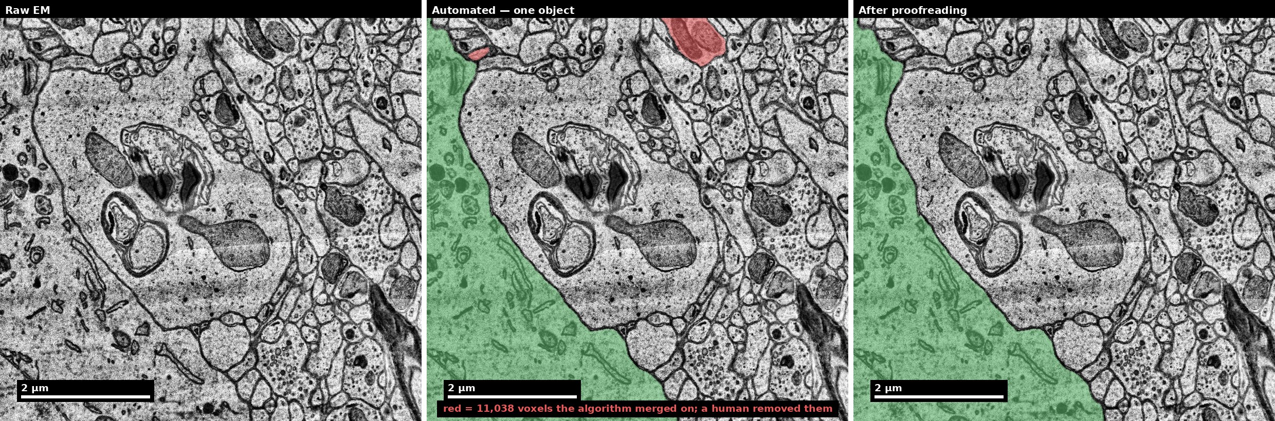Automated segmentation is H01's `c2`; the corrected version is one of its 104 manually proofread cells. Rendered by `scripts/render_em_figures.py`.

False split (over-segmentation)

One continuous cell broken into two or more pieces.

Why it happens. Thin processes — a 60 nm spine neck at 40 nm section thickness may appear in only one or two sections — plus the section artifacts that interrupt continuity: knife chatter, folds, charging and missing sections (Unit 03 §2).

What gives it away:

An ending that is not an ending. A neurite that stops in mid-neuropil without tapering to a natural termination is the classic split candidate, and the one endpoint detectors flag.
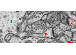
A detached spine head sitting beside a dendritic shaft, with a synapse and nothing connecting it.
Two open ends facing each other across an artifact — a fold, a chatter band, a lost section — with matching calibre and direction.

Correction. Merge the pieces. In a ChunkedGraph system this adds an edge between them; nothing in the image changes.

The same field of human cortex shown twice with segmentation overlaid: on the left the c2 agglomeration labels a region as one object in purple; on the right the c3 agglomeration splits the same region into two objects in red and blue. — Merge or split: the same decision, made two ways. H01 ships two agglomerations of one segmentation. Aggressive c2 (left) calls this region one object; conservative c3 (right) calls it two. If it is really one cell, c3 has made a false split; if two, c2 has made a false merge — and nothing in a single section tells you which. That is the honest limit of this figure: H01 does not say which answer is right for this object, so read it as the diagnosis you would have to make, not as a confirmed split. Across H01's 104 proofread cells, c3 needed 1.6× fewer merge corrections and 2.1× more split corrections than c2. H01 human cortex, Lichtman Lab (Harvard) & Connectomics at Google, CC BY 4.0. Shapson-Coe et al., *Science* 384, eadk4858 (2024). 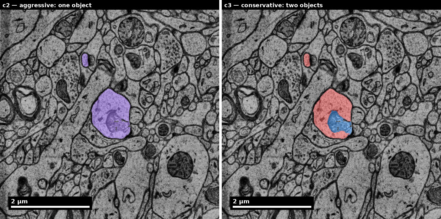Rendered by `scripts/render_em_figures.py`.

Orphan fragment

A piece of segmentation that belongs to no traced object: the far side of a split, left unattached. One orphan costs little. Many of them add up to a large volume of tissue, and synapses, attributed to nobody (Unit 08 §2).

What gives it away. Orphans are easy to count and hard to place. A small object with no soma, both ends open, and a plausible parent passing close by is usually the missing piece of that parent. Find its partner by the split signatures above.

Correction. Merge it into the parent, or, if no parent in the volume fits, record it as unresolved rather than forcing it onto the nearest candidate.

Electron micrograph of a dendrite labelled D with two spines labelled s1 and s2, each opposite a vesicle-filled bouton. — Where orphans come from, not an orphan itself: a dendrite (D) with two spines (s1, s2), each receiving a synapse. If the segmentation loses a thin spine neck, the spine head and its synapse become a separate fragment, and the dendrite's input count drops by one with nothing looking wrong at the dendrite. This site does not yet have a rendered example of a confirmed orphan fragment on real data; the H01 render pipeline that produced the two figures above is where one would come from. Pat Rivlin training materials (MICrONS proofreading deck).

2. Synapse verification criteria

Automated synapse detection is good, and it is not perfect: its misses are not uniform across synapse types, and it transfers imperfectly between datasets (Synapse detection). When you verify a detection, a chemical synapse needs all of the following (Unit 05 §2):

A presynaptic vesicle cluster — vesicles of about 35–50 nm gathered at the membrane facing the partner, not scattered elsewhere in the profile. In flies, the presynaptic side also carries an electron-dense T-bar.
A synaptic cleft — parallel membranes with a uniform gap across the contact, about 20–30 nm at asymmetric synapses and 15–20 nm at symmetric ones, wider than casual membrane apposition.
A postsynaptic density — a dark thickening on the receiving side: pronounced at asymmetric (typically excitatory) synapses, thin at symmetric (typically inhibitory) ones.
Persistence across sections. A synapse is typically 200–500 nm across, so at 40 nm sections a real one appears on two to five consecutive sections. A “synapse” on a single section is one sample of something that should be visible several times.

The commonest false positive is dark contrast alone — a membrane cut at a glancing angle, precipitate, or an adherens junction with symmetric densities on both sides. No vesicles, no synapse.

3. Platform workflows

CAVE and Neuroglancer

The production system behind FlyWire and MICrONS. The segmentation is stored as an editable graph over immutable supervoxels (the PyChunkedGraph), so a merge adds an edge and a split removes one, without rewriting the petascale volume. Every edit is logged with its author and time.

Key bindings differ between Neuroglancer deployments — FlyWire, MICrONS and H01 each run their own — so take them from the deployment’s own help rather than from a list here.

Materialization rule. Never analyse live, unpinned IDs. Pin every query to an explicit materialization version, and put that version in the figure caption and the methods (Unit 04 §2).

webKnossos

An open-source tool for large-scale 3D EM annotation and reconstruction, from the Max Planck Institute and scalable minds (Boergens et al., 2017, Nature Methods 14:691–694). It is built for fast skeleton tracing, including a flight mode for following a process continuously through the volume, and for distributing tracing work as tasks across a team. Skeletons export as NML.

For the wider tool landscape, see Proofreading tools.

4. Community proofreading resources

FlyWire Academy (Princeton) — self-paced videos, interactive worksheets and Python exercises for exploring the whole-brain fly connectome in Codex. Free; Codex needs a Google account.
EyeWire — the Seung lab’s gamified citizen-science platform for tracing neurons in 3D, and a gentle first contact with following a branch and spotting a merge.
CAVEclient documentation — the Python API for querying root IDs, synapse and annotation tables, and edit lineage in CAVE datasets.
SynapseWeb — the Kristen Harris lab’s (UT Austin) online atlas of ultrastructural neurocytology: spines, active zones, PSDs, organelles.
webKnossos user guide — setting up volume layers, sharing annotations, flight-mode tracing and skeleton export.
VAST — the Volume Annotation and Segmentation Tool (Berger et al., 2018, Frontiers in Neural Circuits), for manual and semi-automatic painting of large EM volumes.