The systems that turn a petabyte of EM tiles into a queryable connectome: chunked storage, the alignment and segmentation pipeline, proofreading-safe versioning, and the materialization model that makes analysis reproducible.
Key community resources for this unit:
Neuroglancer The de facto standard open-source WebGL viewer for large-scale volumetric/segmented EM data, used across virtually every major connectomics dataset.
CAVE — Connectome Annotation Versioning Engine
— Dorkenwald et al. (2025), "CAVE: Connectome Annotation Versioning Engine," Nature Methods 22:1112–1120 The annotation/proofreading/versioning backend behind MICrONS, FlyWire, and other large volumes.
BossDB — Brain Observatory Storage Service and Database
— Hider et al. (2022), "The Brain Observatory Storage Service and Database (BossDB): A Cloud-Native Approach for Petascale Neuroscience Discovery," Frontiers in Neuroinformatics Cloud-native storage/serving system built specifically for petascale volumetric EM/connectomics data.
webKnossos
— Boergens et al. (2017), "webKnossos: efficient online 3D data annotation for connectomics," Nature Methods 14:691–694 Open-source tool for large-scale 3D EM annotation and reconstruction (Max Planck / scalable minds).
Before you start
Time
Self-study ~3.5 h: about 2 h of reading plus the 90 min lab. Taught: a 90 min session, per the lecture plan. Deck: the unit’s slide deck is scoped to 60 min and does not follow the plan slide for slide.
Prerequisites
Units 01–03, particularly the data-volume arithmetic
You need
Python with caveclient and cloud-volume installed, or a Colab notebook. A free CAVE account for MICrONS access.
You finish with
A working query against a real petascale volume, pinned to a specific materialization version, plus a capacity plan for a hypothetical new volume
Connectomics infrastructure exists to solve one problem that has no analogue in most
scientific computing: the dataset is simultaneously enormous, mutable, and shared.
A petabyte of images would be easy if nobody edited it. A collaborative editing system
would be easy if the objects were small. Connectomics needs both at once, plus
reproducible analysis on top of an object that changes while you analyze it.
Understanding how that is solved is not optional systems trivia. It determines whether
your analysis is reproducible, and it is the source of the single most common
correctness bug in connectomics papers: results computed against an unpinned,
continuously-edited segmentation.
What you’ll be able to do
Describe the reference pipeline from raw tiles to queryable graph, and say what each stage’s output actually is.
Explain why segmentation is stored as an editable graph over immutable supervoxels, and what that buys.
Explain what a materialization version is and why analysis must be pinned to one.
Query a real petascale dataset and retrieve a neuron’s synapses reproducibly.
Produce a capacity and cost plan for a new volume, with the dominant cost identified.
1. The reference pipeline
Each stage below is a real thing that produces a real artifact. Learn what the
artifact is, because that is what you will debug.
Stage 1 — Ingest
Input: raw tiles from the microscope, plus acquisition metadata.
Output: an immutable, checksummed archive plus a validated tile manifest.
The archive is write-once. Nothing downstream ever modifies it. If a later stage is
wrong, you re-run from here. Treat the raw archive as the only irreplaceable asset in
the project — everything else is recomputable, expensively.
Common failure: metadata that is not machine-readable, so tile position, timestamp,
and acquisition parameters cannot be joined to defects found later.
Stage 2 — Stitching and alignment
Input: tiles.
Output: a coherent 3D image volume, plus the transform stack that produced it.
Two sub-problems:
Stitching (within a section): place tiles relative to each other using their
overlap regions. Mostly rigid or affine per tile.
Alignment (across sections): register section n to section n−1. Hard,
because sections deform non-rigidly — compression from the knife, folds, stretch —
and because errors accumulate. A 0.1-voxel-per-section bias over 20,000 sections is
a 2,000-voxel drift.
Modern pipelines use coarse-to-fine elastic registration with a global relaxation step
that distributes residual error across the whole stack rather than letting it
accumulate in one direction.
What you must retain: the transforms, versioned. Any coordinate you record in the
aligned space is meaningless without knowing which alignment version produced it. When
an alignment is revised, every stored annotation coordinate must be re-mapped — this
is a real and painful operation, and it is why alignment revisions are rare and
carefully planned.
Common failure: alignment residual reported as a global mean. Report the
distribution and the maximum, per region. See Unit 03 §3.
Stage 3 — Boundary/affinity prediction
Input: aligned image.
Output: a per-voxel prediction, same size as the input — either an affinity map
(probability that neighboring voxel pairs belong to the same object, typically in 3
or more directions) or a boundary map.
This is a dense convolutional network applied over petavoxels. It is the most
compute-intensive stage and it is embarrassingly parallel over blocks, with the
important caveat that blocks must overlap, because a network needs context beyond
the region it predicts.
Common failure: block-boundary seams in the prediction, visible later as a regular
grid of segmentation errors. The fix is sufficient overlap plus blending, and the way
you detect it is to look for errors whose spatial distribution matches your block grid
— another instance of the Unit 03 “which coordinate system does the defect live in?”
question.
Stage 4 — Supervoxel generation
Input: affinities.
Output:supervoxels — small, over-segmented fragments, deliberately smaller
than real objects.
This is a design decision with far-reaching consequences. Watershed (or similar) is
run at a threshold that guarantees over-segmentation: a supervoxel may be a piece of a
neurite, but it should almost never span two neurites. The pipeline accepts many
splits in order to avoid merges, because — as Unit 03 argued — merges are the
expensive error.
Supervoxels are immutable. They are the atoms of everything above them. This is
the key to the whole architecture and the next section explains why.
Stage 5 — Agglomeration
Input: supervoxels + affinities (+ increasingly, learned agglomeration models).
Output: the segmentation — an assignment of supervoxels to objects.
Agglomeration merges supervoxels into neurons. Approaches include mean-affinity
agglomeration, learned agglomeration using local shape descriptors, and flood-filling
networks that grow objects iteratively from seeds. What matters architecturally is
that the output is a grouping of immutable atoms, not a new voxel labeling.
Stage 6 — Derived geometry
Input: segmentation.
Output: meshes (multi-LOD, for 3D viewing), skeletons (for morphometry and path
distance), and per-object statistics (volume, surface area, bounding box).
These are regenerated when the segmentation changes, which is constantly. Design them
as cheap, incremental, and per-object.
Stage 7 — Synapse detection
Input: aligned image (and often the segmentation).
Output: a synapse table: coordinates, pre/post supervoxel IDs, confidence,
size/area, and often cleft segmentation.
Modeled as a separate detection problem, usually with its own network. Store
partner identity as supervoxel IDs, not object IDs. Supervoxel IDs are immutable, so
when proofreading changes which neuron an object is, the synapse assignment follows
automatically. Storing object IDs would require rewriting the synapse table on every
edit — a design mistake that is easy to make and painful to undo.
Stage 8 — Annotation and serving
Input: everything above.
Output: interactive viewing (Neuroglancer), proofreading, spatial and relational
queries, and versioned annotation tables.
2. The core idea: an editable graph over immutable atoms
Naive design: store the segmentation as a labeled volume. Then a proofreader merges
two neurons and you rewrite… potentially gigabytes of voxels. With hundreds of
proofreaders editing concurrently, this is unworkable.
The ChunkedGraph solution. Store supervoxels once, immutably. Represent the
segmentation as a graph whose nodes are supervoxels and whose edges are “these are
the same object”. An object is a connected component of that graph. Then:
A merge is adding an edge. Microseconds, not gigabytes.
A split is removing edges — specifically, finding a minimum cut separating two
user-specified points.
The graph is hierarchical and chunked, so connected-component queries over
millions of supervoxels stay fast: the hierarchy lets you answer “what object
contains this supervoxel?” without traversing the whole graph.
Every edit is an entry in an append-only log, with author, timestamp, and
operation. Nothing is destroyed; state at any past time is recoverable.
Concurrent editing works, because edits are small graph operations that can be
applied and reconciled independently.
Systems in production use: CAVE (Connectome Annotation Versioning Engine, used for
MICrONS and FlyWire), DVID, webKnossos, CATMAID (which solved a related
problem for skeleton-based tracing), and neuPrint (a Neo4j-backed graph service
for released, frozen connectomes).
Why this matters to you, the analyst
Because object IDs are not stable. In a ChunkedGraph system, the ID of a neuron
changes every time it is edited. A “root ID” identifies an object as of a moment in
time.
This has a hard consequence: an object ID in your notebook, your paper, or your
figure caption is meaningless without a timestamp or version. This is the number-one
reproducibility failure in connectomics analysis, and it is silent — your code runs
fine, it just answers a different question than it did last week.
Materialization
To make analysis possible at all, the system periodically produces a
materialization: a frozen snapshot in which every annotation (synapses, cell-type
labels, manual annotations) has been joined to the segmentation state at a specific
timestamp, and written into queryable tables.
Analyses run against a materialization version, e.g. version 943.
The version number is a first-class part of your methods section, exactly like a
software version or a genome build.
Re-running the same analysis on a later version will give different numbers,
because proofreading continued. That is correct behavior, not a bug — but it must
be visible.
Rule. Every figure you produce records the materialization version, the query
code, and the date. Every paper states the version. If your collaborator cannot
reproduce your number, the first question is always “which version?”
Worked example: which version produced this number?
The situation: a figure your group submitted eight months ago reports that a
pyramidal cell — root ID quoted in the caption — receives 1,412 input synapses.
Re-running the notebook today returns 1,530 for an ID the lineage viewer says is
“the same cell.” A reviewer asks which number is right.
Step 1 — look for the pin. The notebook has no reproducibility header and the
query does not pass a materialization version. It ran against “latest,” which is
the silent failure this section describes: the code still runs; it now answers a
different question than it did in the winter.
Step 2 — recover the timestamp. The notebook’s commit history dates the run.
That week brackets two materializations — call them 795 and 802 — so the date
alone does not identify the version. This is the uncomfortable part: you are
reconstructing provenance that should have been recorded, from evidence that was
recorded for other reasons.
Step 3 — test both candidates. Pin the query to each version in turn. Version
795 returns 1,412. Exact agreement on the total is suggestive, not conclusive —
two versions could coincidentally match on a sum — so check the per-partner
synapse counts as well. They match row for row. The figure was computed against
795.
Step 4 — explain the difference; don’t just date it. Map the old root ID
forward through the lineage service. It resolves to a single current root — no
splits — but the edit log shows a series of merge operations, each with author and
timestamp, that attached previously split fragments of distal dendrite over the
intervening months. The 118 additional inputs sit on the newly attached arbor.
Both numbers are correct — for different objects. The original claim was
under-specified, not wrong.
Step 5 — repair the record. The response to the reviewer states:
materialization 795, root ID as of that version, n = 1,412; under the current
version the same lineage resolves to a more complete reconstruction with 1,530
inputs. The revised methods section pins the version, and the notebook gains the
five-line header it should have had.
Transferable principle: every provenance question in this system is answerable
because the architecture keeps append-only artifacts — the edit log, the lineage
graph, the materialization snapshots. But answerable-after-an-afternoon-of-forensics
and reproducible-by-construction are different states, and the version number in
the figure caption is what separates them.
Check yourself
Why store synapse partners as supervoxel IDs rather than neuron IDs?
Because supervoxel IDs are immutable and neuron (root) IDs are not.
A synapse is physically attached to a small piece of tissue — a supervoxel. That
attachment never changes, no matter how proofreaders regroup supervoxels into
neurons. So the synapse table is written once and stays correct forever.
If you stored neuron IDs instead, then every merge and split would invalidate rows
in a table with hundreds of millions of entries, and any stale copy of the table
would be silently wrong. Resolving “which neuron does this synapse belong to?”
becomes a lookup from supervoxel → current root at a given version — which is
exactly what the materialization precomputes.
Generalizable principle: in a system with mutable groupings, store foreign keys
against the immutable layer and resolve upward at query time.
Your collaborator sends a list of 200 neuron IDs from six months ago. What do
you do before using them?
Do not query them directly against the current segmentation. Some will no longer
exist; others will have been merged or split, and a stale ID may silently resolve to
something, or to nothing.
The correct procedure:
Ask which materialization version or timestamp the IDs came from. If your
collaborator does not know, that is itself an important finding about the
analysis’s reproducibility.
Use the platform’s ID-lineage facility to map the old root IDs forward to current
root IDs, which will be a one-to-many or many-to-one mapping wherever edits
occurred.
Report the churn. How many IDs mapped 1:1? How many split into several? How
many merged together? That number tells you and your collaborator how much
proofreading changed the objects, and it belongs in the methods.
If the original analysis must be exactly reproduced, query the old version
directly rather than mapping forward.
3. Storage layout, and why chunk shape is a real decision
Petascale volumes are stored as chunked, multi-resolution arrays — the
Neuroglancer precomputed format, N5, Zarr / OME-Zarr, and similar. The recurring
elements:
Chunks: the volume is divided into blocks (commonly 64³ to 512³ voxels) stored
as individual objects. You fetch only the chunks you need.
Resolution pyramid: progressively downsampled copies. Zooming out fetches a
coarse level rather than a million fine chunks. The pyramid costs about 30–50% extra
storage and is what makes interactive viewing possible.
Sharding: millions of tiny objects are slow and expensive in object stores, so
chunks are bundled into larger shard files with an index. This is a pure
cost/latency optimization and it matters a lot at petascale.
Compression: lossy (JPEG) for image data, where a little compression noise is
acceptable; lossless and label-aware (e.g. compressed segmentation) for label data,
where a single flipped bit changes an object’s identity.
Chunk shape is an access-pattern decision, and the two main consumers want opposite
things:
Consumer
Access pattern
Wants
Proofreader in a viewer
Scrolls through z at one xy location, then pans
Chunks elongated in z, or at least isotropic in index space
Analysis job
Reads a whole neuron’s bounding box, or a whole section
Large chunks, sequential layout
Synapse query
Random access to scattered small regions
Small chunks, good spatial index
You cannot optimize for all three with one layout. Production systems store multiple
representations — the image pyramid for viewing, the segmentation graph for editing,
and materialized tables for analysis — precisely so each consumer gets a layout suited
to it. When someone asks “why is this stored three times?”, that is the answer.
4. Reproducibility requirements
A reconstruction pipeline that cannot reproduce its own output is not a scientific
instrument. The requirements are not exotic; they are just rarely all satisfied.
Every stage output records: input artifact IDs, code revision (a commit hash),
full parameter set, model artifact hash and framework version, container image digest,
random seeds, and wall-clock/resource usage.
Idempotency. Re-running a stage on the same inputs with the same parameters
produces the same output. This sounds trivial and is not: GPU non-determinism,
unpinned dependencies, and unseeded randomness all break it. Pin them explicitly and
test that a re-run matches.
Region-scoped invalidation. When a region is re-processed, only downstream
artifacts for that region should be invalidated. A pipeline whose only recovery
option is “re-run everything” cannot fix a local defect at petascale, so this is a
structural requirement, not a nicety.
Release candidates. Segmentation is versioned and released like software: a
candidate is produced, quality metrics are computed (Unit 08), it is reviewed, and it
is either promoted or rejected. Analyses cite the release.
5. Capacity and cost, worked
For a 1 mm³ volume at 4 × 4 × 40 nm (~1.5 × 10¹⁵ voxels):
Item
Estimate
Notes
Raw archive
~1.5 PB
Written once, read rarely; cold storage
Aligned pyramid
~2 PB
Base + ~30–50% for the pyramid; hot
Affinity/boundary maps
~1.5 PB
Often transient — delete after supervoxel generation
Supervoxels + segmentation
~0.2–0.8 PB
Label-aware compression helps a lot
Meshes (all LODs)
1–10 TB
Regenerated on edit
Skeletons
10–100 GB
Cheap; archive them (see Unit 02)
Synapse table
50–200 GB
~5 × 10⁸ rows; the hottest analytical table
Edit history
Grows monotonically
Must be curated, never deleted
GPU cost, order of magnitude. Suppose a segmentation network processes ~10⁷
voxels/second/GPU end-to-end including I/O. For 1.5 × 10¹⁵ voxels:
On 500 GPUs that is roughly 3.5 days of wall clock — and you will run it more than
once, because the first model version is never the last. Budget for 3–5 full inference
passes over the project lifetime.
But the dominant cost is none of the above. It is proofreading labor. At
even a modest few hours of skilled human attention per fully-proofread neuron, a study
needing 1,000 complete neurons is thousands of person-hours. Compute and storage are
line items you can negotiate with a cloud vendor. Proofreading is a hiring, training,
retention, and quality-management problem, and it is the reason Unit 08 spends its
time on triage and prioritization rather than on algorithms.
Cost traps specific to this domain:
Egress. Moving a petabyte out of a cloud region can cost more than storing it
for a year. Co-locate compute with data; give collaborators compute next to the
data rather than copies of it.
Small-object overhead. Billions of unsharded chunks incur per-request charges
and listing costs that can exceed storage costs. Shard.
Forgotten intermediates. Affinity maps are the size of the raw data. Delete them
after supervoxel generation, or set a lifecycle policy — but only once you are
confident you will not need to re-agglomerate.
Idle hot storage. Move the raw archive to cold tiers immediately after ingest
validation.
Check yourself
To cut the storage bill for the 1 mm³ volume above, a colleague proposes one
chunk layout for everything — 64³ chunks, no second representation — serving
proofreading, analysis jobs and synapse queries alike. What goes wrong, and what would
you cut instead?
No single chunk shape serves all three consumers. The §3 table is the argument. Small
isotropic chunks suit the proofreader scrolling through z and the synapse query hitting
scattered small regions, but the analysis job reading a whole neuron’s bounding box
wants large, sequential reads; at 64³ it makes a very large number of small requests,
which in an object store is also the small-object cost trap. The image pyramid, the
segmentation graph and the materialized tables are kept separately so that each
consumer gets a layout suited to it. That duplication is the design, not the waste.
The savings are elsewhere in the same table:
Affinity maps, ~1.5 PB and often transient. Delete them after supervoxel
generation, or put a lifecycle policy on them — once you are confident you will not
re-agglomerate.
The raw archive, ~1.5 PB, written once and read rarely. Move it to cold storage
immediately after ingest validation, but never delete it: it is the only
irreplaceable asset.
Sharding, if the chunks are not already sharded, cuts the per-request charges.
Then say the uncomfortable part out loud: even a perfect storage plan leaves the
dominant cost untouched. Proofreading labor is larger than any of these line items.
Generalizable principle: cut what is recomputable or cold before you cut what
serves a distinct access pattern. The waste is usually an intermediate nobody deleted.
Visual context set
Read these as architecture sketches to check your own mental model against. For each one, ask where the immutable layer sits and where the mutable one does — the whole design in §2 follows from freezing supervoxels and letting only the grouping change.
Module14 L1 S04: A high-level architecture view. Map the eight stages of §1 onto it and name the artifact each stage actually produces, because the artifact is the thing you debug. A stage whose output you cannot name is a stage you do not yet understand.
Module14 L1 S07: Workflow and API integration. Ask what a query crossing these boundaries returns and whether it is pinned: a root ID carries no meaning without a materialization version or timestamp (§2), and this layer is where that omission quietly enters an analysis.
Module14 L1 S12: Service decomposition. Match each service to the consumers in §3 — proofreader, analysis job, synapse query — which want mutually incompatible chunk layouts. Storing the same data in several representations is the answer to “why is this here three times?”, not redundancy.
Module13 L1 S08: Scalable analytics. Weigh whatever scaling story it tells against the cost table in §5: compute and storage are line items you can negotiate with a vendor, and proofreading labor is the dominant cost that no architecture removes.
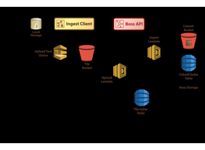
Module14 L1 S14: An ingest path. Tiles leave local storage through an upload queue into a tile bucket with its own index; a second step turns tiles into cuboids — chunks — with a cuboid index. That is Stage 1 and the §3 chunking decision in one picture. Ask where the validated tile manifest lives, and at which arrow the raw tiles become the write-once archive Stage 1 requires.
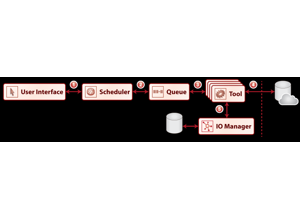
Module13 L1 S12: A job-orchestration loop: interface, scheduler, queue, parallel workers, and an IO manager between the workers and storage. Read it against §4. The queue is where a stage gets re-run, so it is where idempotency is either guaranteed or quietly broken by an unseeded model or an unpinned dependency, and where region-scoped invalidation has to be expressible as a job.
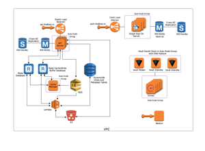
Module14 L1 S05: The service layout of a cloud-hosted volumetric database. Find the object store and the cache in front of it, then apply the §5 cost traps: every chunk fetched is a billed request, so an unsharded layout pays per object, and every byte that leaves the region pays egress. Ask where a collaborator's analysis would run under this layout — next to the data, or on a copy taken out of it.
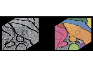
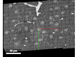
Module14 L1 S09: One slice of a served volume, with a 50 µm scale bar and the viewer's axis lines. A field this wide is what the resolution pyramid in §3 exists for: zoomed out, a viewer fetches a coarse level rather than millions of native-resolution chunks, and the 30–50% extra storage in the §5 table is the price of that.
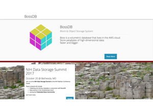
Module14 L1 S19: The public face of one such system: BossDB, which describes itself as a volumetric database in the AWS cloud for petabytes of high-dimensional data (the screenshot is dated by its 2017 banner). Put the §2 question to any service before building on it: does it hold images, a mutable segmentation, or frozen tables — and if a segmentation, where are its versions?
Lab: query a petascale volume reproducibly (90 minutes)
Part A — make a reproducible query (45 min).
Using caveclient against the MICrONS public release (or neuprint-python against
hemibrain, or the FlyWire client, whichever you have access to):
Connect, and print the available materialization versions. Pick one and pin to
it explicitly in your code. Record the version number in a comment at the top of
your notebook.
Pick any neuron. Retrieve its input synapses and its output synapses.
Report: total input count, total output count, and the number of distinct
presynaptic partners.
Compute the distribution of synapses per partner. Note that it is heavy-tailed —
most partners contribute one synapse, a few contribute many. Plot it on log axes.
Now re-run steps 2–4 against a different materialization version. Report how
the numbers changed and explain why.
Write a five-line “reproducibility header” for your notebook: dataset, version,
client library version, date, query author.
Part B — capacity plan (45 min).
Your institute proposes imaging 5 mm³ of mouse hippocampus at 4 × 4 × 40 nm. Produce a
one-page plan:
Raw data volume, computed.
Full storage table (all stages, as in §5), with a stated retention policy for each
line — what is kept forever, what is transient, what is cold.
GPU-days for one full segmentation pass, with your assumed throughput stated. Then
multiply by your assumed number of passes and justify the number.
Proofreading estimate: neurons needed for a stated scientific goal × hours per
neuron × cost per hour. State every assumption.
Identify the dominant cost and defend the ranking.
Name two design decisions that would reduce the dominant cost, and the
scientific price of each.
Rubric
Not yet
Proficient
Strong
Version discipline
No version recorded
Version pinned and reported
Cross-version comparison performed and the difference explained
Query correctness
Runs, unclear result
Correct counts with units
Handles autapses/self-loops, filters by synapse confidence, states the filter
Storage plan
Raw only
All stages, with sizes
Retention policy per line, with cold/hot tiering and egress considered
Compute estimate
Absent
GPU-days computed
Multiple passes justified; failure/re-run budget included
Labor estimate
Absent
Included
Identified as dominant, with assumptions stated and sensitivity noted
Tradeoffs
Generic
Two decisions named
Scientific cost of each decision stated concretely
Hint for Part A step 4, if the distribution surprises you
You should see something close to a power-law-ish, heavy-tailed distribution: a
large majority of partners connect via a single synapse, with a small number of
partners connecting via five, ten, or more.
This shape matters for analysis. Single-synapse connections are exactly the ones
most vulnerable to false-positive synapse detection and to merge errors, so the
“weak” tail of the connectivity distribution is also its least reliable part. Many
analyses therefore apply a threshold (e.g. ≥ 2 or ≥ 3 synapses to call a
connection) — which is a defensible choice that must be stated, because it
changes graph density substantially and it changes it non-uniformly across cell
types. Unit 09 returns to this.
Common errors and how to recover
Unpinned analysis. Recover: pin the materialization version; put it in the
notebook header and the figure caption. Re-run one old analysis with an explicit
version to check you can reproduce it.
Stale object IDs. Recover: map IDs through the lineage service and report churn.
Isotropic assumptions in derived geometry. Recover: check that skeleton path
lengths and distance transforms use physical voxel spacing. Test with a synthetic
object of known dimensions.
Storing derived data keyed on mutable IDs. Recover: re-key to supervoxels, or to
(root ID, version) pairs. Never to a bare root ID.
A pipeline that can only be re-run whole. Recover: introduce region-scoped
artifact keys before you need them. You will need them.
The norm behind this unit
Some of what this unit teaches is technique. Some of it is professional norm — the
things experienced people do without being asked, and which nobody states out loud
because they assume you already know. Those are worth naming, because they are
distributed unequally by background rather
than by ability.
From this unit:
Pin the version, and put it in the figure caption.
An object ID without a materialization version or timestamp is meaningless. This is the most common silent correctness bug in connectomics analysis, and it is invisible — your code still runs.
Treat provenance as a pipeline stage with its own tests.
If the acquisition log is not machine-readable, it does not exist. You will discover this the first time you need to ask whether a defect follows block position or acquisition time.
The collected set, and why making these explicit is a fairness intervention rather than
etiquette, is in the hidden curriculum.
What this unit does not cover
Segmentation model architectures and proofreading practice (Unit 08), the metrics used
to accept a release (Unit 08), and analysis on the resulting graph (Unit 09).
Deployment specifics for any one platform are out of scope — the ideas here transfer
across CAVE, DVID, webKnossos, and neuPrint even though the APIs do not.
Define data lineage fields required for reproducible release.
Propose rollback criteria for failed segmentation updates.
Capability development brief
Capability target: Design a robust ingest-to-serving reconstruction pipeline with reproducibility and rollback controls.
Required expertise
Scientific data engineer (pipeline architecture)
MLOps/platform engineer (orchestration and observability)
Connectomics analyst (task-aware data product requirements)
Core concepts to teach
Data lineage: Traceable provenance from raw imagery through model outputs and manual edits.
SLOs for reconstruction: Target service levels for throughput, latency, integrity, and release cadence.
Versioned releases: Immutable snapshots that allow rollback and cross-analysis reproducibility.
Capability exercise
Pipeline Incident Simulation - Respond to a reconstruction release failure without losing reproducibility. The lab above is the graded version of this exercise; do that one.
Assessment artifacts
Architecture diagram with failure domains and ownership.
Release policy specifying lineage metadata and rollback criteria.
Related concepts
Reconstruction Architecture
Design scalable ingest-to-serving systems with lineage, release, and rollback discipline.