06 Axons and Dendrites

Before you start

Why this needs its own unit. Every edge in a connectome has a direction, and that direction comes from deciding which process was the axon. Get it backwards and you have not added noise — you have added a confidently wrong, oppositely directed edge. In a downstream motif analysis, a reversed edge converts a feedforward chain into a recurrent loop. There is no statistical correction for this after the fact.

The added difficulty is that in dense neuropil you usually cannot reach a soma. The process enters your field of view, crosses it, and leaves. Classification has to work from local evidence.

What you’ll be able to do

1. Classify a neuronal process as axonal or dendritic from local evidence, with a stated confidence.
2. Name the four exceptions where the polarity rule fails, and recognize when you are in one.
3. Explain why direction errors cost more than identity errors, quantitatively.
4. Measure your own agreement against a reference and identify which cue you over-trust.
5. Write a classification protocol that another annotator can follow to comparable agreement.

1. The cue table

Organized by the Unit 05 cue families, because independence is what determines confidence.

Family A — organelle content

Family B — geometry and caliber

The taper rule is more useful than it looks. At a dendritic branch point, the cross-sectional areas of the daughters are systematically smaller than the parent. At an axonal branch point, caliber is roughly preserved. When you can see a branch point, this is a Family B cue that is fully independent of organelle staining quality — which makes it valuable exactly when Family A is unreliable.

Family C — synaptic polarity

The default rule:

• The process bearing the vesicle cluster at a synapse is presynaptic → axonal.
• The process bearing the PSD is postsynaptic → dendritic or somatic.

This resolves most cases and is why finding a single clean synapse on a process is often worth more than a long scroll.

Family D — context and destination

• Position within a myelinated bundle or a fiber tract → axon.
• Wrapped by an oligodendrocyte sheath → axon.
• Arising from a soma with an AIS (membrane undercoating plus fasciculated microtubules, roughly 20–60 µm long) → axon, definitively.
• Arising from a soma with a broad base, tapering, and containing ribosomes → dendrite, definitively.
• Following the process to any soma is the gold standard, when the volume allows.

2. The exceptions that break the polarity rule

Family C is powerful and it is not universal. You must be able to recognize the situations where it fails, because applying it blindly there produces confident, systematic, direction-reversing errors.

1. Dendro-dendritic synapses. In the olfactory bulb, mitral/tufted cell dendrites and granule cell dendrites form reciprocal synapses with each other — vesicle clusters in a dendrite. Also present in the thalamus (interneuron presynaptic dendrites) and elsewhere. If you are annotating olfactory bulb or thalamus, the polarity rule is not a safe default.

2. Axo-axonic synapses. Chandelier cells synapse onto the axon initial segment of pyramidal cells. Here the postsynaptic element is an axon. If you find a PSD on a process, that does not by itself prove dendrite — check whether you are on an AIS (undercoating, fasciculated microtubules, proximity to a soma).

3. Presynaptic dendrites in retina. Amacrine cells make output synapses from processes that are not conventional axons. In retina, the axon/dendrite dichotomy is partly the wrong frame.

4. Invertebrate neurons. In Drosophila and C. elegans, many neurons are unipolar with mixed input/output regions on the same neurite. The “axon” and “dendrite” labels are approximations applied to compartments of a single process, and polarity must be assessed synapse by synapse rather than process by process.

The practical rule. Before applying the polarity rule as a default, ask: what tissue am I in? Cortex, hippocampus, and cerebellum are mostly well-behaved. Olfactory bulb, thalamus, and retina are not. Invertebrate brains need a different frame entirely. This is a question about the dataset, not the image, and it should be answered once, in the protocol, rather than repeatedly by each annotator.

Check yourself

3. The local classification protocol

Use when you cannot reach a soma — which is most of the time.

1. Is there a synapse on this process, anywhere in view?
   YES -> which side is it on?
      Vesicle cluster on this process  -> AXON (confidence: high)
      PSD on this process              -> DENDRITE or AIS
                                          -> check for undercoating +
                                             fasciculated microtubules
                                          -> and check tissue type against
                                             the exception list (Sec. 2)
   NO  -> continue

2. Are ribosomes visible?
   YES -> DENDRITE (confidence: high)
   NO  -> weak evidence only; absence at this caliber may just mean
          the process is too thin. Continue.

3. Is there myelin, or is the process inside a fiber bundle?
   YES -> AXON (high)

4. Follow through z for at least 2-3 um and check:
   - Beaded with discrete vesicle-bearing swellings?     -> AXON
   - Steady taper, or a branch with thinner daughters?   -> DENDRITE
   - A spine emerging?                                   -> DENDRITE (high)

5. Still unresolved -> UNCERTAIN.
   Record which cue was missing and why. Route to the review queue.

Note what step 2’s “NO” branch says. Absence of ribosomes is weak evidence, because a 150 nm process may simply be too thin to contain a visible polyribosome in this plane. Absence is only evidence when the feature would have been visible if present. Beginners routinely over-read absence, and it is worth calling out explicitly during training.

Worked example: a 200 nm process, no soma in reach

Patch: cortical neuropil. An unbroken process, roughly 200 nm across, enters the field, runs about 4 µm, and leaves. Staining is moderate. No soma is reachable — the standard situation this protocol exists for.

Tissue check first (§2): cortex, so the polarity rule is a safe default here. Answered once, from the protocol, not re-litigated per process.

Step 1 — synapse in view? Not on the first pass through the visible stretch. Continue.

Step 2 — ribosomes? None visible. The tempting move is to lean axon — but at 200 nm the process may simply be too thin to show a polyribosome in any one plane, so this absence is weak evidence, exactly as the note above warns. Record it; do not spend it.

Step 3 — myelin or fiber bundle? No. Continue.

Step 4 — follow through z. Over about 3 µm the process holds its thin caliber, then swells once, discretely, and narrows again — beaded rather than tapering, which is Family B evidence for axon. Inside the swelling, small round profiles. Vesicles, or a grazing cut through something else? In this single section, genuinely unsure. Two sections further on, the ambiguity resolves: the round profiles cluster against an apposition with a bulbous partner, and the partner carries a dark thickening on its side — a PSD, persistent across sections.

That is step 1 answered late: a vesicle cluster on this process, PSD on the partner. Presynaptic role — Family C.

Call: axon — an en passant bouton onto a probable spine head. Confidence: high. Evidence chain: Family B (constant intervaricose caliber with one discrete vesicle-bearing swelling; no taper over 3 µm) plus Family C (presynaptic role at a persistent synapse). Two independent families, continuity confirmed — high tier under the Unit 05 definitions.

Worth recording is what stayed out of the chain: thinness (caliber alone is the cue this unit’s lab most often catches people over-trusting, and it would only duplicate Family B), and the ribosome absence from step 2, which never became evidence because it was unresolvable at this diameter.

Transferable principle: the protocol’s order is a cost order, and it loops — cheap checks first, then z-continuity, which frequently hands you the step 1 answer you did not have at the start. One clean synapse settled in three sections what organelle evidence could not settle in four micrometers, and the discipline is refusing the cheap caliber call while you look for it. For the same protocol run to the opposite verdict — a dendrite call assembled over four passes — see the extended worked case in Axon–dendrite classification.

4. Why direction errors cost more: the arithmetic

Suppose you classify 1,000 processes with 95% accuracy — 50 errors.

• If the errors were identity errors (right direction, wrong cell), you would lose 50 edges and gain 50 wrong ones. Bad, but the graph’s directional structure is intact.
• Because they are direction errors, each one removes an edge in the true direction and adds one in the reverse direction. The effect on any direction-sensitive statistic is doubled.

Now consider what this does to a reciprocity measurement. Take a population with a true reciprocal-pair rate of 5%. Flip the direction of a random 5% of edges. Some flips convert one-directional pairs into reciprocal pairs. The measured reciprocity rises, and it rises in the direction that makes the result look more interesting, because “reciprocal connections are enriched” is a publishable finding and “reciprocity is at chance” is not.

This is a bias, not noise, and it points toward the exciting answer. That is the worst possible property for an error to have.

Mitigations that work:

1. Report classification confidence per edge, and re-run the headline analysis restricted to high-confidence edges. If the effect survives, say so. If it does not, you have learned the most important thing about your result.
2. Prefer within-dataset comparisons where the error rate is shared between the groups being compared, so it partly cancels.
3. Estimate the error rate directly on a gold-standard subset and propagate it — simulate the effect of that error rate on your statistic and report the resulting uncertainty band.
4. Audit asymmetrically. Spend review effort on edges whose direction changes the conclusion, not uniformly across all edges.

Visual training set

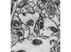
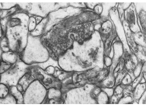
Use these with the protocol in §3 in hand, and force yourself to name the step that resolved each case — or the step at which you stopped. They are single planes, which is the habit to break: steps 4 and 5 both require following a process for micrometers through z. Treat the panel as a reference for what each cue looks like rather than as a surface you can classify from.

RIV-AXDEN S01: Orientation for the axon-versus-dendrite comparison. Fix the four cue families first — organelle content, caliber geometry, synaptic polarity, context — because confidence here comes from which families agree, not from how many observations of the same kind you stack up.

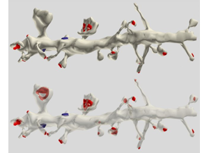
RIV-AXDEN S08: A dendrite-focused cue. Look for the geometry evidence that survives bad staining: steady taper with distance from soma, and daughter branches thinner than the parent at a branch point. That taper rule is independent of stain quality, which makes it valuable exactly when the ribosome cue has failed you.

RIV-AXDEN S11: Classification in dense neuropil — the normal case, where no soma is reachable. Run step 1 of the protocol first: a single clean synapse anywhere in view settles polarity faster than a long scroll, and the side carrying the vesicle cluster is the axon.

RIV-AXDEN S13: A side-by-side comparison. Name three differences, label each with its family, then ask which of them you would still see at ten percent weaker membrane contrast. That ordering is your personal cue-robustness ranking, and the calibration lab is where you measure it.

RIV-AXDEN S14: An ambiguity case. Resist stacking more of the same evidence: high confidence requires two cues from different families. If everything available belongs to one family, the honest output is medium confidence with the missing family named.

RIV-AXDEN S18: An edge case. Before applying “PSD implies dendrite”, check the exception list in §2 — an axon initial segment receiving chandelier input is postsynaptic and still an axon. The tell is membrane undercoating plus fasciculated microtubules within roughly 20–60 µm of a soma.

Attribution: Pat Rivlin training materials (MICrONS proofreading deck). Some manifest-listed IDs used in planning (`S04`, `S06`, `S10`, `S16`) were not present in extracted thumbnails and were replaced with available neighboring cues.

Lab: calibration round (90 minutes)

The goal is not to get the answers right. It is to measure your error profile so you know which cues you personally over-trust.

Setup. You need a patch set of 20 processes with reference labels. Build one from a public volume by selecting processes that can be traced to a soma (so ground truth exists) but presenting only a local crop to the learner. Include:

• 8 straightforward cases (4 axon, 4 dendrite)
• 6 hard cases (thin processes, poor local contrast, no visible synapse)
• 4 exception cases (at least one AIS receiving a synapse)
• 2 cases that are actually merge errors

Procedure.

1. Round 1, independent. Classify all 20. For each, record: call, confidence tier, the cue you relied on most, and its family.
2. Score. Compute overall accuracy, and accuracy by confidence tier.
3. The key diagnostic — calibration. Of the calls you marked high confidence, what fraction were correct? If high-confidence accuracy is well below ~90%, you are overconfident, and that is a more important finding than your overall score.
4. Error analysis by cue. For each error, which cue misled you? Tabulate. Most people find one cue dominates their errors — commonly caliber, which is a Family B cue that beginners treat as if it were Family A.
5. Round 2, paired. With a partner, re-do the 6 hard cases. Discuss before committing. Record whether discussion changed either call and why.
6. Protocol writing. Together, write a one-page classification protocol that would have prevented your most common error. Be specific: “when caliber is the only available cue, mark uncertain” is a usable rule; “be careful with caliber” is not.

Rubric

Common errors and how to recover

Treating caliber as a primary cue. It is Family B and it is context-dependent. Recover: rule that caliber alone never supports a high-confidence call.

Applying the polarity rule outside cortex. Recover: put the tissue-specific exception list at the top of the annotation protocol, not in a footnote.

Over-reading absence. Recover: add “was the feature resolvable here?” as an explicit step before treating absence as evidence.

Missing merge errors because the cues “mostly agree”. Recover: treat any high-reliability cue conflict as a merge alarm and inspect the path.

Uniform review effort. Recover: prioritize review by whether the edge’s direction affects a conclusion.

The norm behind this unit

Some of what this unit teaches is technique. Some of it is professional norm — the things experienced people do without being asked, and which nobody states out loud because they assume you already know. Those are worth naming, because they are distributed unequally by background rather than by ability.

From this unit:

• Report confidence per call, then re-run the headline result on high-confidence calls only. If the effect survives, say so. If it does not, you have learned the most important thing about your result — and reporting that is what distinguishes a careful analyst.

• Choose the cheaper error deliberately, and say that you did. Biasing yourself toward the recoverable mistake is not sloppiness; it is an asymmetric loss function applied on purpose. Say so, or it reads as carelessness.

The collected set, and why making these explicit is a fairness intervention rather than etiquette, is in the hidden curriculum.

What this unit does not cover

Glial processes, which are the other major source of thin-process confusion and are covered in Unit 07. Also not covered: how these classifications enter proofreading prioritization (Unit 08) or motif analysis (Unit 09).

Go deeper

• Axon–dendrite classification — extended cue reference with worked cases
• Axon biology — AIS, boutons, conduction, and the biology behind the cues
• Dendrite biology — spines, shafts, and integration
• Myelin and nodes of Ranvier — myelin as a classification cue
• Neuron type identification — from process class to cell type

Course links

• Reading list: Technical Track Journal Club
• Shared vocabulary: Connectomics Dictionary
• Related modules: Module 04, Module 09
• Lecture plan: Axons and Dendrites lecture plan
• Next unit: 07 Glia