What a synapse-resolution wiring diagram can and cannot tell you, and how to turn a broad brain question into a measurable connectomics study.
Key community resources for this unit:
White, Southgate, Thomson & Brenner (1986)
— "The Structure of the Nervous System of the Nematode Caenorhabditis elegans," Phil. Trans. R. Soc. Lond. B 314(1165):1–340 The founding connectome paper — the first complete synaptic wiring diagram of an animal nervous system (C. elegans).
Bargmann & Marder (2013)
— "From the connectome to brain function," Nature Methods 10:483–490 Directly addresses what a structural wiring diagram can and cannot tell you about function — the core question this unit asks.
Sporns, Tononi & Kötter (2005)
— "The Human Connectome: A Structural Description of the Human Brain," PLoS Computational Biology 1(4):e42 The paper that coined "connectome" and framed the field's motivating agenda.
Sebastian Seung, Connectome: How the Brain's Wiring Makes Us Who We Are
Popular-science framing of the field's motivation and stakes, by a leading connectomics researcher (Houghton Mifflin Harcourt, 2012).
Before you start
Time
Self-study ~2.5 h: about 90 min of reading plus the 60 min lab. Taught: an 85 min session, per the lecture plan. Deck: the unit’s slide deck is scoped to 60 min and does not follow the plan slide for slide.
Prerequisites
None
You need
Paper or a text editor. No data or code.
You finish with
A one-page study brief for a connectomics question of your own
This unit is deliberately not about microscopes. It is about the reasoning step that
happens before anyone buys a microscope, and that most failed connectomics projects
skip: deciding what claim the data will be asked to support.
What you’ll be able to do
By the end of this unit you should be able to:
State, from memory, what physical features require electron-microscopy resolution and why light microscopy cannot substitute.
Estimate the raw data volume of a proposed EM experiment to within an order of magnitude, given a target tissue volume and voxel size.
Classify a connectivity claim as supported by structure alone, supported by structure plus an extra assumption, or not supportable by structure.
Convert a vague biological interest into a study brief containing a measurable structural endpoint, a null model, and an explicit non-claim.
Item 3 is the one that matters most. It is also the one most often failed.
1. The resolution argument, in numbers
Connectomics exists because of a physical mismatch between the size of the things
that carry information in the brain and the resolution of the instruments that are
cheap and fast.
Structure
Approximate size
Resolvable by light microscopy (~200–250 nm limit)?
Cortical neuron soma
10–25 µm
Yes, easily
Dendritic shaft
0.5–3 µm
Yes
Myelinated axon
0.5–2 µm
Usually
Dendritic spine head
300–800 nm
Marginally
Unmyelinated axon in neuropil
80–300 nm
No
Dendritic spine neck
50–200 nm
No
Synaptic cleft
~20 nm
No
Synaptic vesicle
~40 nm
No
Postsynaptic density
30–50 nm thick
No
The consequence is specific, not general. Light microscopy can tell you that two
neurons’ arbors overlap in space. It cannot tell you whether they are connected,
because at 250 nm two membranes 20 nm apart are one blur. In dense cortical neuropil,
a 1 µm³ box contains on the order of a dozen distinct neurites; below the diffraction
limit they are indistinguishable.
Electron microscopy at 4 nm × 4 nm × 40 nm resolves all of the rows above. That is the
entire reason the field tolerates the cost described in the next section.
A caution that belongs here and not later. Resolving a synapse is not the same as
knowing its sign, strength, or whether it is active in a behaving animal. EM gives
you an anatomical synapse: a presynaptic vesicle pool, a cleft, and a postsynaptic
specialization. Sign (excitatory/inhibitory) is usually inferred from morphology
(see Unit 05) or from a separate molecular measurement, not read off directly.
Check yourself
A colleague proposes using confocal microscopy of sparsely labeled neurons to
"map the connectome" of a cortical column. What is the strongest single objection?
Sparse labeling plus diffraction-limited optics gives potential contact (arbor
overlap), not synaptic connection. Contact-based predictions of connectivity —
“Peters’ rule” style inference — are known to be poor predictors of actual synaptic
connectivity in cortex: neurons that touch frequently often do not connect, and
connection probability varies strongly by cell type. You would be measuring a
proxy whose relationship to the quantity of interest is itself an open research
question.
A secondary objection: sparse labeling means you cannot see the unlabeled
partner, so even a true synapse has an anonymous other side.
2. The cost argument, in numbers you can compute
You should be able to do this arithmetic in your head, because it is the fastest way
to sanity-check any proposal.
Raw voxel count = (volume) ÷ (voxel volume).
Work an example. Take 1 mm³ of cortex at 4 nm × 4 nm × 40 nm:
x: 1 mm / 4 nm    = 1,000,000 nm / 4 nm    = 250,000 voxels
y: 1 mm / 4 nm    =                          250,000 voxels
z: 1 mm / 40 nm   = 1,000,000 nm / 40 nm  =  25,000 voxels

total = 250,000 x 250,000 x 25,000 = 1.56 x 10^15 voxels
At 8-bit grayscale that is ~1.56 petabytes of raw image data for one cubic
millimeter — before alignment, before segmentation, before meshes, before any
derived product. Published petascale volumes land in this range: the H01 human
temporal cortex sample and the MICrONS mouse visual cortex volume are both roughly
one cubic millimeter and both are reported in the 1.4–2 PB range depending on what is
counted and how it is compressed.
Now extrapolate, and notice where it breaks:
Target
Volume
Raw data at 4×4×40 nm
Status
C. elegans nervous system
~0.00005 mm³
~0.1 TB
Done, repeatedly, since 1986
Adult Drosophila brain
~0.02–0.03 mm³
~40 TB
Done (FAFB / FlyWire, hemibrain)
Mouse cortical column / 1 mm³
1 mm³
~1.6 PB
Done (MICrONS)
Whole mouse brain
~500 mm³
~800 PB
The current grand challenge
Whole human brain
~1.2 × 10⁶ mm³
~10²¹ bytes
Not a plan; a horizon
Teaching point. The jump from fly to mouse cortex is ~40×. The jump from 1 mm³ to
whole mouse brain is ~500×, and it is not a jump in imaging alone — it is a jump in
sectioning reliability, storage economics, alignment robustness, segmentation
accuracy, and above all proofreading labor. Programs such as NIH BRAIN CONNECTS
exist because that 500× is an engineering problem, not a microscopy problem.
Check yourself
You are offered beam time to image 0.05 mm³ of mouse hippocampus at
isotropic 8 nm (FIB-SEM). How much raw data, roughly, and what changes relative to
4×4×40 nm?
What changes: isotropy. At 4 × 4 × 40 nm the z-axis is 10× coarser than xy, so thin
processes running in-plane are easy and processes crossing z steeply are hard —
this anisotropy is the single largest driver of automated segmentation errors
(Unit 08). Isotropic 8 nm removes that asymmetry, at the cost of throughput and of
a hard limit on how large a volume FIB-SEM can practically mill.
3. What structure can and cannot establish
This is the section to argue about. Sort every claim you plan to make into one of
three bins.
Bin A — structure alone is sufficient evidence
“Neuron X makes 42 synapses onto neuron Y.” Direct anatomical observation.
“Cell type A targets the proximal dendrites of type B, while type C targets distal
dendrites.” Compartment-targeting is measured, not inferred.
“Reciprocal pairs occur 4× more often than expected under a degree-preserving null
model.” A structural statistic against a stated null.
“This projection does not exist in this volume.” A negative result, with a stated
detection sensitivity.
Bin B — structure plus one declared assumption
“This synapse is excitatory.” Requires the assumption that asymmetric
(Gray type I) morphology predicts glutamatergic transmission. Usually a good
assumption in cortex; it is still an assumption, and it fails for known exceptions.
“This is a strong connection.” Requires assuming synapse count or total
postsynaptic-density area is monotonic in physiological strength. Defensible, and
supported in some systems, but it is a model.
“This circuit performs coincidence detection.” Requires a biophysical model
linking morphology and connectivity to integration.
Rule: any Bin B claim must name its assumption in the same sentence, or in the
figure caption. “Putatively excitatory (asymmetric morphology)” costs four words.
Bin C — structure cannot establish this
“This circuit computes X during behavior Y.” Requires physiology.
“This synapse is potentiated.” Requires a functional or molecular measure.
“This wiring causes the animal’s decision.” Requires perturbation.
“Neuromodulatory state Z reconfigures this circuit.” Volume transmission is
largely invisible in a standard EM volume.
A wiring diagram is a constraint on the space of possible dynamics, not a
simulation. The most common failure of connectomics writing is a Bin C sentence in
the abstract supported by a Bin A measurement in the results.
Worked example: repairing a research question
Version 0 (as originally proposed): “We will use connectomics to understand how
the cortex implements predictive coding.”
This is Bin C, it has no measurable endpoint, and no result could falsify it.
Repair it in four moves.
Move 1 — find the structural signature. Predictive-coding architectures generally
require some form of asymmetry between feedforward and feedback pathways, and a
population that receives both. In mouse visual cortex, a candidate structural
signature is: feedback axons from higher visual areas preferentially target a
different dendritic compartment of layer 2/3 pyramidal cells than feedforward
thalamocortical and layer 4 inputs do.
Move 2 — define the measurement, with units. For each proofread L2/3 pyramidal
cell, compute the fraction of input synapses by presynaptic source class, binned by
path distance from soma (0–50, 50–150, 150–300, >300 µm) and by compartment (spine
head, spine neck, shaft, soma, AIS). Report as synapses per source class per
compartment per cell, n cells.
Move 3 — state the null. Sources are distributed across compartments in
proportion to available postsynaptic surface area in each compartment. This null is
important: dendrites have more distal surface than proximal, so “more distal
synapses” is the expected result and is not evidence of anything.
Move 4 — write the non-claim. “These data constrain where feedback input arrives
on the dendritic tree. They do not establish that these synapses carry prediction
error signals, and they do not establish sign; sign is inferred from synaptic
morphology and from the identified source cell type.”
Version 1 (usable): “In mouse visual cortex, do inter-areal feedback axons
target a systematically more distal dendritic compartment of L2/3 pyramidal cells
than L4 feedforward axons do, relative to a surface-area-proportional null,
measured across ≥50 proofread cells?”
Version 1 can be answered, can be wrong, and can be scoped in a grant.
Check yourself
Sort these into Bin A / B / C.
(i) "The mushroom body Kenyon cell input is random with respect to glomerular identity."
(ii) "This interneuron inhibits pyramidal cell firing."
(iii) "Layer 5 thick-tufted cells receive 3× more synapses on their apical tuft than
layer 5 slender-tufted cells."
(i) Bin A, provided “random” is defined against a stated null model and the
claim is restricted to the reconstructed population. It becomes Bin B if it is
extended to “input is unstructured”, since unstructured with respect to one
labeling scheme may be structured with respect to another.
(ii) Bin B, verging on C. “Is GABAergic and forms symmetric synapses onto the
pyramidal cell’s soma and proximal dendrite” is Bin A/B. “Inhibits firing” is a
functional claim; a GABAergic synapse can be depolarizing depending on chloride
reversal potential and developmental stage. State it as “putatively inhibitory”.
(iii) Bin A, and note that it is a ratio, which quietly controls for a lot of
reconstruction bias. Ratios between comparably reconstructed populations are more
robust than absolute counts, which are sensitive to completeness. This is a habit
worth acquiring early.
4. Sizing the claim to the reconstruction
A structural claim is only as good as the completeness of the reconstruction behind
it. Match the claim type to the reconstruction state you actually have:
Claim type
Minimum reconstruction state
Typical failure if you skip this
“Cell X synapses onto cell Y”
Both partners proofread through the synapse; synapse manually verified
A merge error invents the connection
“Cell X has n inputs”
Full dendritic arbor proofread and closed
Split errors truncate the arbor; n is an undercount of unknown size
“Type A prefers type B over type C”
Both target populations proofread to comparable completeness
Differential completeness masquerades as biological preference
“Motif M is enriched”
A closed subgraph with quantified edge precision/recall
False edges from merges inflate dense motifs superlinearly
“This projection is absent”
Stated detection sensitivity and searched volume
Absence of evidence reported as evidence of absence
The fourth row deserves emphasis and reappears in Unit 09: merge errors do not add
noise symmetrically to motif counts. A single merge fuses two neurons’ partner
lists, which manufactures triangles and reciprocal pairs at a rate far above the
error rate itself. Motif analysis on unproofread segmentation is not conservative;
it is biased in a specific and predictable direction.
5. What connectomics has actually delivered
Concrete anchors, so that “connectomics is useful” is a claim you can defend with
examples rather than enthusiasm.
C. elegans, 302 neurons (White et al. 1986; Cook et al. 2019; Witvliet et al.
2021). The first complete nervous system. Its lasting lesson is negative and
useful: having the complete wiring diagram of 302 neurons did not immediately
yield an understanding of behavior. It took decades of physiology and genetics on
top of the map. Witvliet’s developmental series added something the single adult
map could not — which connections are stable across maturation and which are not.
Adult Drosophila (hemibrain, ~25,000 neurons; FlyWire whole brain, ~139,000
neurons and ~54.5 million synapses). The first whole-brain connectome of an animal
with complex behavior. It produced genuinely new biology: complete cell-type
censuses, the wiring of the central complex as a ring-attractor navigation system,
and connectome-constrained network models that predicted taste and behavioral
responses which were then tested experimentally.
MICrONS, ~1 mm³ mouse visual cortex (~200,000 cells, ~500 million synapses),
with two-photon functional imaging of the same tissue. The important thing here is
not size; it is the co-registration. Structure and function in the same neurons is
what lets you ask whether wiring predicts tuning — and the answer so far is
“partially, with cell-type-specific rules”, which is exactly the kind of result that
only this data type can produce.
H01, ~1 mm³ human temporal cortex (~57,000 cells, ~150 million synapses).
Demonstrated that human tissue obtained surgically can be prepared and reconstructed
at this scale, and immediately surfaced features rare or absent in mouse, such as
axons forming dozens of synapses onto a single target.
Note what is common to the useful results: each one is a census or a comparison,
not an assertion about computation. That is the shape of a defensible connectomics
result today.
Visual context set
These five slides are framing devices, not evidence. Use each one to rehearse the sort in §3: for whatever claim the slide invites, ask whether structure alone could establish it, whether it needs a declared assumption, or whether it needs physiology the data does not contain.
Techtalk S10: The motivating question, asked before any instrument is chosen. Use it to practice the move this unit is built on — name the measurable structural endpoint, the null model, and the explicit non-claim that would have to replace it before the question is fundable.
Techtalk S11: Framing for what counts as brain data. Read it against the resolution table in §1: for whatever measurement the slide treats as data, ask which rows of that table it resolves, and therefore whether it can distinguish arbor overlap from an actual connection.
Techtalk S12: The reverse-engineering analogy, and where it stops. Check it against the bin boundaries in §3 — a wiring diagram is a constraint on the space of possible dynamics, not a simulation, so any “this circuit computes X” reading of the analogy is a Bin C claim wearing Bin A clothing.
Module12 L1 S04: Scope framing for the course. Compare whatever ambition it states against the extrapolation table in §2, and ask where on the fly-to-mouse-to-human ladder it lands — and whether the limiting factor at that rung is microscopy or proofreading labor.
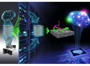
Module12 L1 S07: The whole pipeline as one illustration: tissue and microscope, image stack, compute, reconstructed neurons — and a final arrow to a brain drawn over a chip. Sort the arrows with §3. Everything up to the reconstruction is structure. The last arrow is a claim about computation, and it stays in Bin C until someone names the assumption that would carry it.
Attribution: neuroAI and outreach source decks (historical/context visuals).
Lab: write a study brief (60 minutes)
Deliverable: one page. Produce it in this order; do not skip to the method.
Biological question (2–3 sentences). Must contain a noun phrase naming a
structure and a verb phrase naming a relationship.
Structural signature. What would have to be true of the wiring if your
hypothesis were correct? What would have to be true if it were false? If you cannot
answer the second, stop and reframe — an unfalsifiable signature is the most common
defect at this step.
Three measurements, with units. For example: synapses per connected pair
(count); fraction of output synapses onto spines vs shafts (dimensionless ratio);
path length from soma to synapse (µm). “Connectivity” is not a measurement.
Dataset requirements. Voxel size; volume; species and age; required
completeness (fragments / neurite-level / near-complete local circuit); estimated
raw data volume computed as in §2.
One null model, stated precisely enough that someone else could implement it.
One confound you cannot remove, and how you will report it.
One non-claim — a sentence you will not write, in quotation marks, with the
reason.
Rubric
Not yet
Proficient
Strong
Falsifiability
No stated outcome would disconfirm the hypothesis
A disconfirming outcome is named
Disconfirming outcome named and distinguished from “underpowered”
Measurement
Named qualitatively (“look at connectivity”)
Three measurements with units
Measurements chosen at the right scale for the hypothesis (local motif claims use local statistics, not whole-graph summaries)
Null model
Absent, or “compare to random”
A named null
Null preserves the nuisance structure that matters (degree, distance, cell-type composition)
Scope discipline
Bin C claims present
Non-claim stated
Bin B assumptions named inline where they occur
Feasibility
No data estimate
Volume and voxel size given
Data estimate computed, and proofreading effort acknowledged as the binding constraint
Self-grading tip: the single best predictor of a weak brief is that step 7 is
empty or vague. If you cannot name a sentence you refuse to write, you have not yet
found the boundary of your evidence.
Common errors and how to recover
“We’ll figure out the analysis once we have the data.”
Recover by writing the figure caption for your main result now, with fake numbers.
If you cannot write the caption, the experiment is not specified.
Using whole-graph summary statistics to test a local hypothesis.
Mean path length and global clustering coefficient are nearly useless for claims about
a specific microcircuit, and they are highly sensitive to reconstruction errors. If
the hypothesis is about a three-cell motif, measure the three-cell motif.
Treating a reconstruction boundary as a biological boundary.
Neurons cut by the volume edge have truncated arbors. Any per-cell count is biased
downward, and the bias is worse for cells near the edge and for cell types with large
arbors. Either restrict analysis to cells whose relevant arbor is fully contained, or
model the truncation explicitly.
Comparing populations that were proofread differently.
If population A was proofread to completion and population B was not, every
difference you find is confounded with effort. Match proofreading protocol before
comparing, and report proofreading state per cell.
The norm behind this unit
Some of what this unit teaches is technique. Some of it is professional norm — the
things experienced people do without being asked, and which nobody states out loud
because they assume you already know. Those are worth naming, because they are
distributed unequally by background rather
than by ability.
From this unit:
Name the assumption in the same sentence as the claim.
“Putatively excitatory (asymmetric morphology)” costs four words. Writing “excitatory” instead is not a shorthand; it is a different claim.
Write down the sentence you refuse to write.
Every study brief should carry an explicit non-claim. Reviewers read it as confidence, not weakness — but nobody tells you that, so most people leave it blank.
Prefer ratios to absolute counts when comparing.
A ratio between comparably reconstructed populations quietly controls for a great deal of reconstruction bias. Experienced people reach for it automatically.
The collected set, and why making these explicit is a fairness intervention rather than
etiquette, is in the hidden curriculum.
What this unit does not cover
Imaging physics (Unit 03), segmentation methods (Unit 08), and the statistics of
motif testing (Unit 09). It also does not cover non-EM connectomics — barcoding
approaches such as MAPseq/BARseq, and diffusion MRI tractography — which answer
different questions at different scales; see Unit 02 for how these fit together.
Go deeper
Connectome history — Cajal through BRAIN CONNECTS, with the lessons from each era
NeuroAI bridge — structure-function relationships and honest boundaries
Quantitative scientist (hypothesis testing and null models)
Core concepts to teach
Structural hypothesis: A claim that predicts measurable wiring patterns, not just broad functional outcomes.
Evidence boundary: A pre-declared limit on what the data can and cannot support.
Null model: A baseline connectivity expectation used to test whether observed motifs are enriched.
Capability exercise
From Question to Test - Convert an aspirational idea into a measurable connectomics plan. The lab above is the graded version of this exercise; do that one.
Assessment artifacts
One-page study brief with question, measurable outputs, and non-claims.
Metric table linking each claim to required structural evidence.
Related concepts
Hypothesis Framing
Translate broad brain questions into testable structural hypotheses with clear evidence boundaries.