How to choose a modality, resolution, and representation for a connectomics question, and how to link measurements across scales without over-claiming.
Key community resources for this unit:
Lichtman, Pfister & Shavit (2014)
— "The big data challenges of connectomics," Nature Neuroscience 17:1448–1454 Contrasts data scale, resolution, and volume tradeoffs across the imaging modalities used in connectomics.
Human Connectome Project The canonical large-scale MRI-based structural/functional connectivity dataset — the macro-scale anchor point against light-microscopy and EM.
Allen Brain Map Allen Institute's multi-modal, multi-scale brain data portal. The institute hosts several distinct sub-portals (Allen Brain Atlas, Allen Brain Cell Atlas, Allen Brain Observatory) — check which sub-resource best fits before linking deeper than the main portal.
Before you start
Time
Self-study ~2.75 h: about 90 min of reading plus the 75 min lab. Taught: a 90 min session, per the lecture plan. Deck: the unit’s slide deck is scoped to 60 min and does not follow the plan slide for slide.
Prerequisites
Unit 01 — specifically the voxel-count arithmetic in §2
You need
A calculator. Optional: a Neuroglancer link to any public volume
You finish with
A scale-selection memo defending one modality choice against two alternatives
Almost every practical connectomics decision is a scale decision in disguise. “Should
we use SBEM or ssTEM?” is a scale decision. “Can we answer this with the existing
public dataset?” is a scale decision. “Why doesn’t our tractography result match the
EM result?” is a scale decision that was made badly, earlier.
What you’ll be able to do
Place any neuroscience measurement modality on a resolution/volume/throughput chart from memory, within an order of magnitude.
Given a biological question, name the smallest sufficient resolution and justify why the next step coarser fails.
Choose among volume, mesh, skeleton, and graph representations for a given analysis, and state what each discards.
Describe how a claim measured at one scale can and cannot be transferred to another.
Detect “scale leakage” — a mechanistic claim resting on data that cannot resolve the mechanism — in someone else’s writing and in your own.
1. The three scales that are not the same thing
Practitioners routinely conflate three different scales. Separating them prevents most
downstream confusion.
Acquisition scale — the voxel size and field of view your instrument produces.
Set by physics and budget. Fixed once the data exists.
Reconstruction scale — the smallest object you can reliably segment. This is
always coarser than acquisition scale, sometimes much coarser. At 4 × 4 × 40 nm you
acquire enough signal to see a 20 nm cleft, but the objects you can segment reliably
are neurites down to roughly 50–100 nm, and the reliability drops sharply for
processes running steeply through z.
Analysis scale — the unit your conclusions are about: a synapse, a cell, a cell
type, a layer, an area, a projection.
The decision rule. Choose the coarsest acquisition scale whose reconstruction
scale still resolves every object your analysis scale depends on. Not the finest
you can afford — the coarsest that works. Every step finer multiplies data volume,
alignment difficulty, and proofreading hours.
A worked instance of the rule: if your endpoint is “fraction of inputs onto spines vs
shafts”, your analysis scale is the synapse and the spine neck. Spine necks are
50–200 nm. So your reconstruction scale must be ≤ 50 nm, which forces EM. If instead
your endpoint is “does area A project to area B at all”, your analysis scale is the
axon bundle, and light-sheet imaging of a bulk tracer at 1 µm is not merely adequate —
it is the correct choice, because it costs about five orders of magnitude less.
2. The modality chart
Learn this table. Ranges are typical rather than record-setting.
Modality
Resolution (typical)
Practical volume
What it uniquely gives you
What it cannot do
Diffusion MRI tractography
0.5–2 mm
Whole human brain, in vivo
Whole-brain, living, repeatable, human
Cannot see individual axons; produces false and missing tracts; no synapses; no direction
Light-sheet / whole-brain LM with tracers
0.5–2 µm (xy)
Whole mouse brain
Long-range projection maps, many animals
Cannot resolve neurites in neuropil; no synapses
Confocal / two-photon
200–300 nm lateral
mm³, in vivo possible
Function (calcium), molecular labels, live
Diffraction-limited; overlap ≠ connection
Expansion microscopy
~25–70 nm effective
Up to ~mm³ with effort
Molecular identity plus near-EM geometry
Expansion distortion; not yet routine for dense reconstruction at scale
Array tomography
~50–100 nm lateral, 70 nm sections
~10⁵ µm³
Multiplexed protein labeling with synapse-scale geometry
Section loss; lower z-resolution than EM
Barcoded projection mapping (MAPseq/BARseq)
Single-cell identity, no geometry
Whole brain, 10⁴–10⁶ cells
Projection patterns of enormous numbers of individual cells, cheaply
Resolution, volume, and throughput form a budget you cannot escape: you may choose
two. FIB-SEM buys resolution and gives up volume. Light-sheet buys volume and
throughput and gives up resolution. Multibeam ssSEM is the current attempt to buy
resolution and volume by throwing an unreasonable amount of throughput engineering at
the problem — 61 or 91 beams in parallel — and it is why 1 mm³ became feasible.
Check yourself
You want to know whether individual layer 2/3 neurons in mouse visual cortex
that project to area AL also project to area PM, across thousands of cells. Which
modality, and why not EM?
Barcoded projection mapping (MAPseq/BARseq). The question is about
single-cell projection classes across thousands of cells — it needs statistical
power over cells, not geometry within a cell. MAPseq delivers exactly that at a
cost per cell that is orders of magnitude below EM.
EM is the wrong tool here for two reasons: (1) a 1 mm³ EM volume does not contain
both AL and PM plus the V1 somata, so you would need a much larger volume than is
currently feasible; (2) even if it did, the answer needs n in the thousands, and
EM proofreading of thousands of complete long-range axons is not tractable today.
The honest limitation to state: barcoding gives you projection presence in a
target region, not synapses in that region, and it is vulnerable to
fibers-of-passage and to barcode-sharing artifacts.
A tractography paper reports a "structural connection" between two regions.
An EM study of one of those regions finds no axons from the other. Both can be
correct. Explain.
They are measuring different things at scales that do not nest cleanly.
Tractography infers streamlines from voxel-scale water diffusion orientation. A
streamline is a model output, not an observed axon. Known failure modes include
false continuations at crossing-fiber regions and difficulty entering gyral crowns.
A tractography “connection” is a statement about the most probable pathway given a
diffusion model — it is not a claim that a specific axon terminates there.
Meanwhile, an EM volume samples a small region. Absence of axons in that volume is
evidence about that volume, at whatever detection sensitivity the reconstruction
achieved. If the projection terminates in an adjacent layer or a neighboring
column, EM would miss it.
The resolution is not “one of them is wrong”. It is that neither claim, as usually
written, states its sampling and its inference model clearly enough to be compared.
This is scale leakage in both directions.
3. Representations: what each one throws away
After reconstruction, the same neuron exists in four representations. Choosing wrongly
is a common and expensive mistake because conversions are lossy and usually one-way.
Representation
What it is
Keeps
Discards
Typical size, one cortical neuron
Volume / labeled voxels
The segmentation itself
Everything, including membrane geometry and organelles
Surface detail, spine head shape, membrane apposition
0.1–5 MB
Connectivity graph
Nodes = cells, edges = synapse counts
Who connects to whom, how strongly
All geometry — compartment, distance, position
Bytes per neuron
The rule that saves projects: decide which representation your endpoint metric
requires before the pipeline runs, and keep the next-richer one archived.
Concrete example of getting this wrong: a team exports a connectivity graph, runs
motif analysis, and finds an enrichment. A reviewer asks whether the enrichment is
explained by spatial proximity — dendrites that are close connect more. The graph has
no geometry, so the question cannot be answered without re-running from skeletons.
Archiving skeletons alongside the graph costs a few gigabytes and prevents this
entirely.
Which representation for which question
“How many synapses between A and B?” → graph
“Where on the dendrite do those synapses land?” → skeleton (path distance from soma) + synapse coordinates
“Are spines on this dendrite larger than on that one?” → mesh
“Is this a merge error?” → volume, always. Every proofreading decision ultimately returns to the voxels.
Worked example: choosing a representation for an inhibition-distance question
Question as posed: “On layer 2/3 pyramidal cells, do putatively inhibitory
(symmetric) synapses sit closer to the soma, in path distance, than putatively
excitatory (asymmetric) ones?” Planned scope: ~300 proofread cells from an
existing public volume.
Start from the endpoint, not from what the pipeline happens to emit. The
measurement is a distribution of path distance from soma, per synapse, per synapse
class. Now hold each representation against that requirement.
Graph: discards all geometry, including the one quantity the question is
about. Rejected in one line.
Volume: contains everything, at GB per neuron — order 1 TB of hot label data
for 300 cells — and computing path distance from voxels means extracting a
centerline anyway. You would be building skeletons expensively, on demand, forever.
Mesh: 10–100 MB per neuron, so 3–30 GB for the study. Surfaces are the right
tool for spine shape, which this endpoint does not need, and path distance along
the arbor is not a natural mesh operation.
Skeleton plus synapse coordinates: 0.1–5 MB per neuron — 30 MB to 1.5 GB for
all 300 cells — and path distance from soma is the native query on a centerline
graph. This is exactly the pairing the list above prescribes for “where on the
dendrite do those synapses land?”
So far the decision looks free. Here is where it is not. Skeletons discard spine
geometry, so a synapse on a spine head gets mapped to the nearest shaft node, and
its path distance loses the neck. Asymmetric synapses land mostly on spines;
symmetric ones mostly on shafts and somata (Unit 05). The shortening therefore
falls mostly on one of the two classes being compared — a differential bias, the
dangerous kind. How large is it? The skeleton cannot tell you; it discarded
precisely that quantity. Probably small against distance bins tens of micrometers
wide — but “probably” is not a number you can print.
The resolution is the archiving rule from this section: run the analysis on
skeletons, and archive the meshes — 3–30 GB, noise next to the roughly 2 PB
aligned pyramid the volume already carries. On a 20-cell subsample, measure the
spine-neck offset on the mesh, and either correct the distances or report the
bound.
Transferable principle: choose the representation whose native operation is
your endpoint metric; reject the coarser candidates by naming the discarded
quantity that disqualifies them; and archive the next-richer representation
specifically so you can bound the bias the one you chose introduces.
4. Cross-scale linkage: registration and its residuals
Linking scales — EM to two-photon function, EM to a reference atlas, one animal to
another — is registration, and registration is where confident-looking errors are
manufactured.
The pipeline
Choose anchors. Vasculature is the best anchor for EM↔LM in cortex: it is
sparse, high-contrast in both modalities, distributed throughout the volume, and
biologically stable within an animal. Soma positions are second best. Layer
boundaries are a weak anchor — they are gradual and observer-dependent.
Fit a transform, of the lowest complexity that works. Rigid → affine →
non-linear, in that order. Reach for a non-linear warp only when residuals demand
it, because a sufficiently flexible warp will align anything, including things
that do not correspond.
Report residuals locally, not globally. A mean residual of 3 µm over the whole
volume can hide a 40 µm error in one corner. Report a residual map or, at minimum,
per-region residual distributions with the maximum.
Hold out anchors. Fit on a subset, measure residuals on anchors the fit never
saw. A model evaluated on its own training points reports its flexibility, not its
accuracy.
Propagate the uncertainty. If EM↔functional registration has 5 µm local
residual and you are assigning calcium traces to somata that are 15 µm across and
sometimes 10 µm apart, some assignments are wrong. Quantify how many, and carry
that number into the result.
Anisotropy warning. On a 4 × 4 × 40 nm stack, an isotropic Gaussian smoothing
kernel, an isotropic distance metric, or an isotropic morphological operation is
silently wrong by a factor of 10 in z. Check every library call for whether it takes
voxel spacing. This bug is common, quiet, and it biases every distance-based
measurement you make.
Check yourself
Your EM↔two-photon registration reports mean residual 2.1 µm, max 31 µm.
Should you proceed to assign functional traces to reconstructed cells?
Not globally, and not yet. The max tells you there is a region where the transform
fails. Steps, in order:
Map residuals spatially. A 31 µm error is almost never uniform noise — it is a
region (often a volume edge, a tissue fold, or a poorly-anchored depth) where
the transform extrapolates.
Decide whether to exclude that region or add anchors there.
For the regions you keep, compute a per-cell assignment confidence using the
local residual and the local soma density. Where nearest-neighbor soma
spacing is comparable to local residual, mark assignments ambiguous rather than
forcing a match.
Report the number of cells excluded and the number ambiguous. A functional
connectomics result whose paper does not state its registration residual
distribution has not shown its work.
5. Compute and storage, planned rather than discovered
Storage for the raw volume is the smallest line item. Plan for the multiplier.
For a 1 mm³ ssTEM volume (~1.6 PB raw), typical derived footprints:
Aligned image pyramid (multi-resolution, for interactive viewing): +30–50% of raw
Affinity / boundary predictions at full resolution: ~1× raw (often float, then quantized)
Segmentation labels (64-bit IDs, compressed): 0.1–0.5× raw
Proofreading edit history and versioned materializations: grows without bound and must be curated
The operational lesson: the raw volume is written once and read rarely. The synapse
table and the segmentation are read constantly, by many people, with latency
expectations measured in milliseconds. Budget for query load, not just capacity.
A petabyte in cold object storage is cheap; a 200 GB table that must answer 50
concurrent interactive queries is the part that needs engineering. Unit 04 covers the
architecture that follows from this.
Visual context set
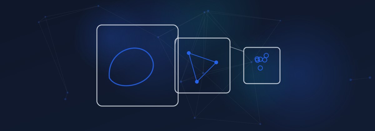
Use this panel to rehearse the three-scale separation from §1. For each slide, say which scale it is actually about — acquisition, reconstruction, or analysis — because pipeline diagrams routinely blur all three, and noticing the blur is the skill this unit is teaching.
Module12 L1 S06: Voxel size and scale. Whatever resolution the slide names, run it through the decision rule in §1: reconstruction scale is always coarser than acquisition scale, so ask what the smallest reliably segmentable object would be rather than what the voxel size implies.
Module12 L2 S04: A macroscale pipeline. Place it on the modality chart in §2 and name which two corners of the resolution/volume/throughput triangle it buys — and therefore which one it gives up. Nothing at macroscale resolves neurites in neuropil, so connectivity read off it is model output, not observation.
Module12 L2 S05: The bridge from macroscale to microscale. This is exactly where scale leakage is manufactured: check what claim is being carried across the join, and whether the transfer comes with a stated registration residual and its maximum, not just its mean (§4).
Module12 L3 S08: High-throughput imaging. Ask what representation the output eventually becomes — volume, mesh, skeleton, or graph (§3) — because that decision is effectively made here, and every conversion downstream is lossy and one-way.
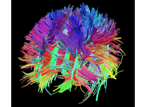
Module12 L3 S03: Whole-brain diffusion tractography. Place it on the modality chart in §2 — 0.5–2 mm resolution, whole living human brain — and read its last column: no individual axons, no synapses, no direction. Every coloured line is a streamline, a model output, which is the whole of the answer to the tractography check-yourself in §2.
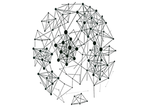
Module12 L2 S06: A network drawing: nodes, edges, and clusters. This is the connectivity-graph row of the §3 table, the smallest representation and the one that discards all geometry. Before trusting any cluster in a picture like this, ask the reviewer's question from §3: would proximity alone explain it, and is there a richer representation archived to check?
Scenario. Your lab wants to test whether inhibitory interneurons in mouse visual
cortex preferentially target the axon initial segment (AIS) of pyramidal neurons that
share functional tuning, versus pyramidal neurons that do not.
Write a two-page memo that selects a data strategy. Required sections:
Decompose the question. List every physical object your endpoint depends on.
(Hint: there are at least four, and one of them is not anatomical.)
Minimum resolution, defended. For each object, the size and therefore the
required reconstruction scale. Then state explicitly what fails if you go one step
coarser.
Modality choice, with two rejected alternatives. For each rejection, name the
specific structure it would fail to resolve or the specific measurement it could
not make. “Too low resolution” is not a reason; “cannot resolve a 1 µm AIS
segment’s synaptic input, and cannot distinguish symmetric from asymmetric
synapses” is.
Cross-scale plan. How functional tuning gets linked to reconstructed cells:
anchors, transform class, residual target, and holdout validation.
Representations. Which representation each of your three measurements comes
from, and what you will archive.
Budget estimate. Raw volume by the Unit 01 arithmetic, plus a derived-product
multiplier, plus an estimate of proofreading hours with your stated assumption
about hours per neuron.
The bottleneck. Name the single step most likely to end the project, and one
mitigation.
Rubric
Not yet
Proficient
Strong
Decomposition
Question restated
All required objects listed with sizes
Includes the non-anatomical requirement (functional tuning) and notes it forces in-vivo imaging before fixation
Resolution defense
Asserts EM
States required scale per object
States what specifically fails one step coarser, per object
Rejections
Alternatives listed
Rejected with a reason
Rejected with the specific unresolvable structure named
Registration
Mentioned
Anchors and transform named
Residual target, holdout plan, and consequence of failure quantified
Budget
Absent
Raw volume computed
Derived products and proofreading labor included; labor identified as dominant
Bottleneck
Generic (“funding”)
A real pipeline step
A step with a stated failure probability and a concrete mitigation
Sample answer sketch for step 1 (open only after attempting it)
Objects the endpoint depends on:
The AIS — a ~20–60 µm segment of proximal axon, identifiable in EM by its
membrane undercoating and fascicled microtubules. Requires EM; it is not
distinguishable from proximal dendrite in LM without a molecular label.
Synapses onto the AIS — chandelier-cell cartridges, symmetric. Requires
≤ 50 nm to identify and to classify as symmetric.
Identity of the presynaptic interneuron — requires tracing the axon back to a
soma with enough arbor to type the cell. This is the expensive part: it needs a
proofread axon, not just a synapse detection.
Functional tuning of the postsynaptic pyramidal cell — not anatomical.
Requires two-photon calcium imaging of the same tissue before fixation, hence the
whole experiment must be planned as a functional-then-structural pipeline, with
registration as a first-class design constraint rather than an afterthought.
The point of the exercise: step 4 changes the entire project structure and is the
thing most often discovered too late.
Common errors and how to recover
Scale leakage. A mechanistic claim resting on data that cannot resolve the
mechanism. Recovery: write the sentence, then write underneath it the smallest object
the sentence depends on, then check that object against your reconstruction scale.
Trusting a global registration metric. Recovery: always produce a residual map.
If your tooling does not produce one, produce it manually from held-out anchors.
One-way representation conversion. Recovery: archive the next-richer
representation. Skeletons alongside graphs; meshes alongside skeletons if storage
allows.
Isotropic operations on anisotropic data. Recovery: audit every distance,
smoothing, and morphology call for voxel-spacing arguments. Add a unit test that
computes a known distance along z.
Assuming public data fits your question. Recovery: before proposing new
acquisition, check whether MICrONS, FlyWire, H01, or a BossDB volume already contains
the objects you need at the scale you need. Frequently one does, and the honest answer
to “what modality?” is “none — this is a re-analysis”.
The norm behind this unit
Some of what this unit teaches is technique. Some of it is professional norm — the
things experienced people do without being asked, and which nobody states out loud
because they assume you already know. Those are worth naming, because they are
distributed unequally by background rather
than by ability.
From this unit:
Report registration residuals locally, with the maximum — never as a global mean.
A mean residual of 3 µm can hide a 40 µm failure in one corner. A reader who knows the field looks for the distribution first and distrusts a paper that reports only the mean.
Archive the next-richer representation.
Keeping skeletons alongside a connectivity graph costs a few gigabytes and answers the reviewer question you cannot otherwise answer without re-running the pipeline.
The collected set, and why making these explicit is a fairness intervention rather than
etiquette, is in the hidden curriculum.
What this unit does not cover
The physics of image formation and the artifact catalog (Unit 03), the systems
architecture that stores and serves these representations (Unit 04), and the
statistics that operate on the resulting graph (Unit 09).
Cross-scale linkage: Anchoring micron-to-nanometer information using shared landmarks or priors.
Capability exercise
Multiscale Design Exercise - Pick the smallest sufficient dataset design for a defined question. The lab above is the graded version of this exercise; do that one.
Assessment artifacts
Scale selection memo with justification and risk analysis.
Data budget estimate (storage, throughput, annotation effort).
Related concepts
Scale Selection
Choose imaging and analysis scale that can resolve required features at manageable cost.