
H01, Step by Step
The H01 case study tells you what H01 is. This page is the other half: how it was made, one stage at a time, and what each stage actually costs.
H01 is a roughly cubic-millimetre fragment of human temporal cortex, imaged by serial-section electron microscopy and reconstructed computationally — a collaboration between the Lichtman laboratory at Harvard and the Connectomics at Google team, published in Science in May 2024.
Every electron-microscopy figure here was rendered directly from the public H01 volume — the same data you can open yourself. Nothing is an artist’s impression. How the figures were made gives you the code.
Before you quote a number from this page
H01’s official sources give different values for the same quantity, because they count different things at different pipeline stages. Getting this wrong is the easiest mistake to make about this dataset, so here are the ones that matter:
| Quantity | Correct value | The number people get wrong |
|---|---|---|
| Physical sections cut | 5,019 (mean thickness 33.9 nm) | “5,293” — that is the digital layer count. About 5.8% of cuts came out double-thickness, and those are duplicated in the stack to keep the z-geometry honest. |
| Data volume | 1.8 PB raw acquisition; 1.4 PB aligned volume | The two get conflated constantly. Say which you mean. |
| Synapses | 149,871,669 found (paper) | The release site says “183 million annotated” — a different product of a different agglomeration. Both are real; cite the source. |
| Cells | 57,180 total = 49,080 neurons and glia + 8,100 blood-vessel-related | The Explore page rounds to “over 50,000”. |
| Proofread cells | 104 | The landing page rounds to “100”. |
Where this page states a number, it is the Science paper’s figure unless it says otherwise. Two habits worth forming: cite the paper’s numbers when you cite the paper, and the release page’s numbers when you describe the downloadable data — and never average them.
The scale problem, first
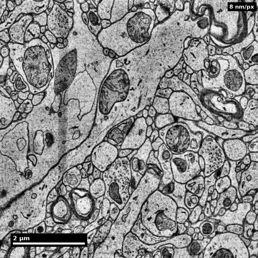
Before the pipeline makes sense, you need to feel the range it spans. These views are all the same tissue, each roughly 4× closer than the last.
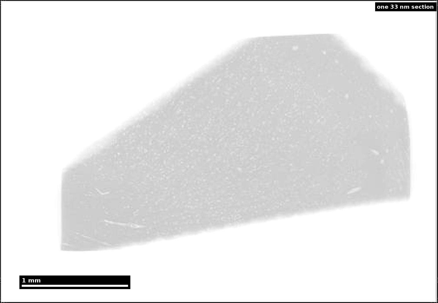
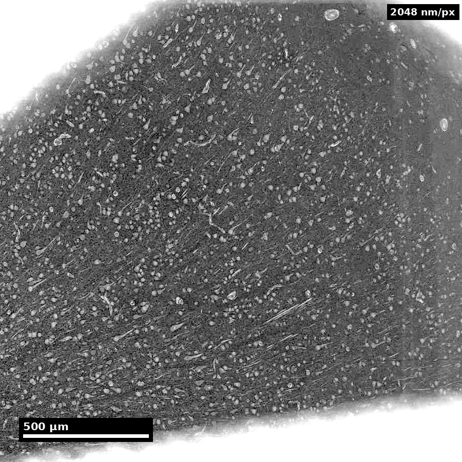
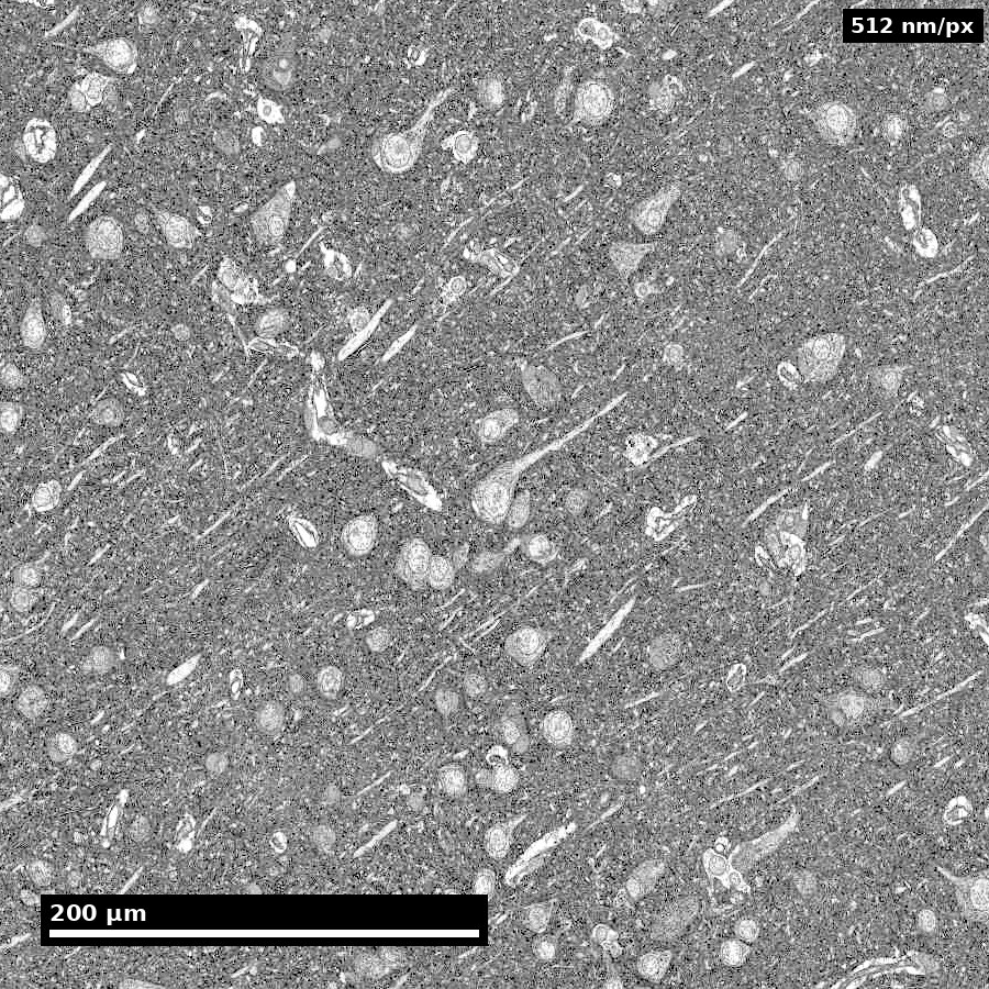
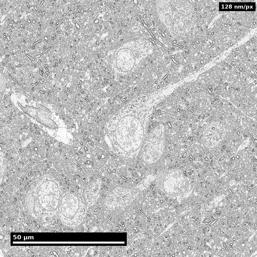
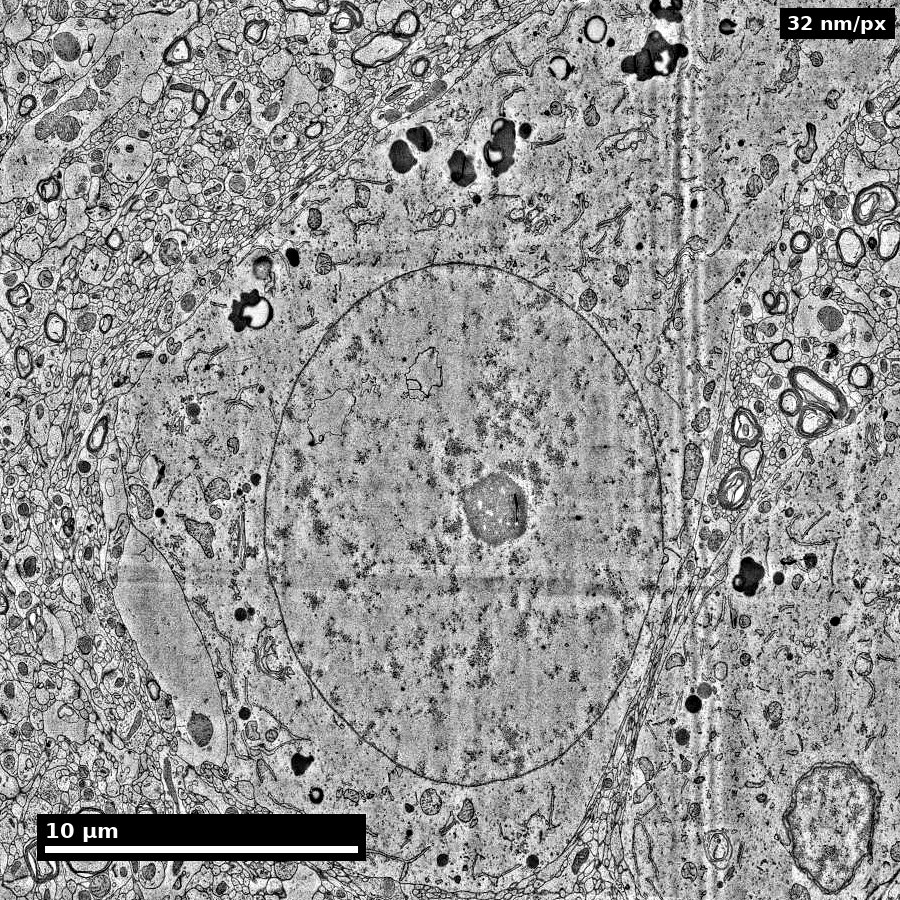
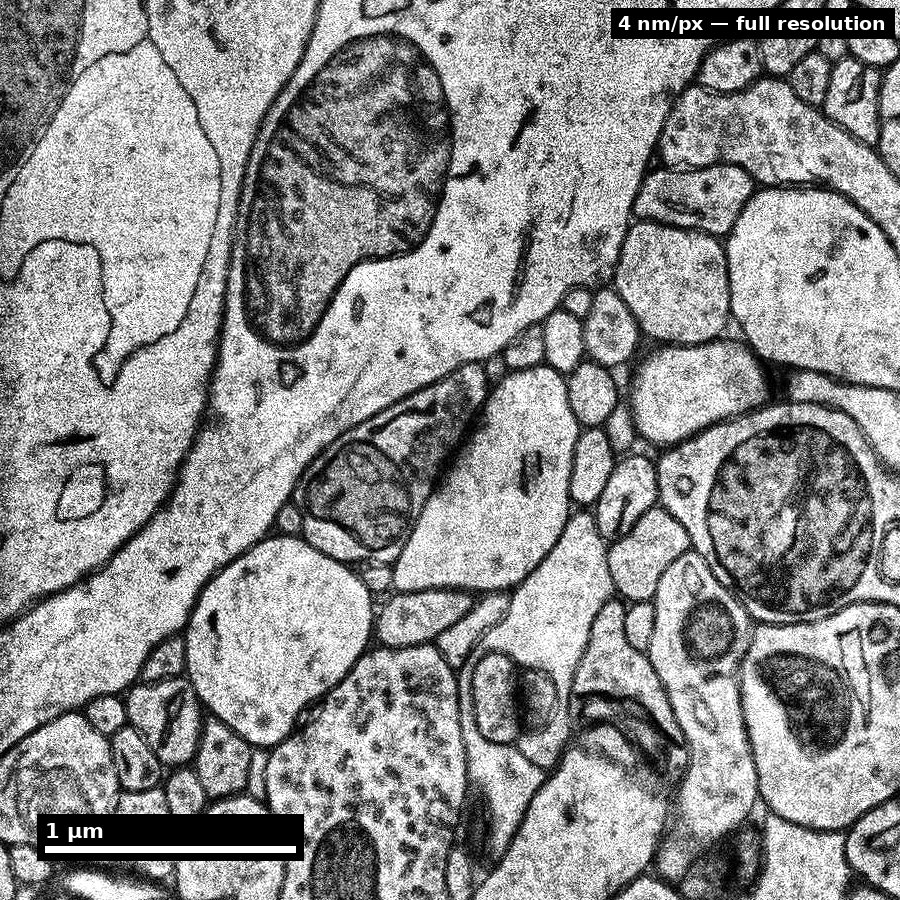
That last step is the whole problem in one image. To find synapses you need this resolution, and you need it everywhere, across a volume 4 mm wide. That ratio is why H01 took 1.8 petabytes and 326 days of microscope time.
Step 1 — The tissue
The sample is human, and that shapes everything downstream.
It is a slab of anterior middle temporal gyrus, about 170 µm thick and spanning all six cortical layers plus white matter — roughly 3 mm from layer 1 to white matter. It was removed during surgery to reach an epileptic focus in the underlying hippocampus in a patient with drug-resistant epilepsy: tissue that had to come out to get access, and would otherwise have been discarded.
Neuropathological examination found the reconstructed piece to be normal by light microscopy — it specifically lacked the aggregated layer-2 neuron band seen when epilepsy-associated hippocampal sclerosis extends into the adjacent temporal lobe. (The resected medial temporal lobe did show hippocampal sclerosis; the anterior temporal piece that became H01 did not.)
Two consequences to hold onto:
- Fixation speed governs everything. Human surgical tissue cannot be perfusion-fixed the way an anaesthetised mouse can; it was immersion-fixed immediately after excision. The authors’ conclusion is genuinely encouraging for the field: sample quality was “comparable to cardiac perfused rodent samples,” which suggests rapid immersion is a viable alternative to perfusion.
- It is one specimen, from one person, with a neurological condition. There is no second human cubic millimetre to compare it against.
Step 2 — Fixation, staining, and embedding
Electrons do not see soft biological membranes on their own. Every step here converts wet tissue into a hard block whose membranes scatter electrons.
- Fixation — immersion in cold 2.5% paraformaldehyde / 2.5% glutaraldehyde in 0.1 M sodium cacodylate buffer, cross-linking proteins and locking structure in place.
- Heavy-metal staining — a ROTO protocol (reduced osmium / thiocarbohydrazide / osmium), following Tapia et al., Nature Protocols 7, 193–206 (2012), followed by en bloc uranyl acetate. This is what actually creates contrast: everything dark in the figures above is, physically, heavy metal deposited on membrane.
- Dehydration and embedding — an ethanol series, then propylene oxide, then infiltration with Epon resin and curing at 60 °C, producing a block hard enough to cut at tens of nanometres without tearing.
The governing trade-off: stronger staining gives better membrane contrast and easier automated segmentation, but pushed too far it obscures the intracellular detail — vesicles, organelles — that you also need.
Depth on this stage: the tissue preparation and EM principles entries cover the chemistry and the contrast physics, and Unit 03 works through the whole preparation chain and the artifacts it produces.
Step 3 — Sectioning
The block was cut into an ordered series of ultrathin sections using an automated tape-collecting ultramicrotome (ATUM), which collects the ribbon of sections onto tape rather than requiring each to be handled individually.
- 5,019 sections, mean thickness 33.9 nm (92.5% between 30 and 33 nm)
- total sample thickness 0.170 mm
- sections mounted onto silicon wafers, ~110–135 sections per wafer
Two facts make this the most fragile stage in the pipeline:
Sections are irreplaceable. A destroyed section is a permanent gap — you cannot re-cut it, because the block face has moved past it. H01’s own cutting history shows what that means in practice: cutting became unstable after ~1,639 sections and the knife had to be replaced; the replacement sat non-parallel to the block face, producing a run of partial “reentry” sections before full sections resumed. Estimated permanent loss across that episode: no more than the equivalent of three 30 nm sections.
Cuts get missed. About 5.8% of sections came out double-thickness (60–66 nm), meaning a cut was skipped. Rather than pretend otherwise, those are duplicated in the digital stack so the z-geometry stays physically honest — which is why the released volume has 5,293 layers but only 5,019 physical sections were cut. If you have seen “~5,300 sections” quoted, that is where it comes from, and it is the layer count, not the section count.
Sectioning also compressed the tissue 28% in the cutting direction. The corrected in-plane pixel size is therefore 5.55 × 4 nm, and the uncompressed tissue volume works out to about 1.05 mm³.
Section thickness is the anisotropy you fight forever after. H01's voxels are 4 × 4 × 33 nm — roughly 8× coarser through the block than within a section. Every downstream algorithm has to cope with that, and it is the main reason a thin process can be followed confidently within a section but lost between them.
Step 4 — Imaging
Sections were imaged on a Zeiss multibeam SEM (mSEM) that scans with 61 electron beams in parallel, covering a hexagonal field of about 10,000 µm² at once, at 4 × 4 nm per pixel.
The arithmetic is the point:
| Beams | 61, in parallel |
| Throughput | 125–190 million pixels/second (most data at 190 M px/s) |
| Raw data per section | up to 350 GB |
| Total imaging time | 326 days |
| Raw data acquired | 1.8 petabytes, 247 million image tiles |
| Tiles containing cortex, stitched and aligned | 196 million |
| Aligned output volume | 1.4 petabytes |
At single-beam SEM throughput, this volume would take longer than a research career. Parallel-beam imaging is the entire reason petascale volume EM is feasible at all — and even so, 326 days is most of a year of continuous microscope time.
A custom workflow manager assessed every tile for quality during acquisition, detecting focus failures, stage-settling artifacts and charging, and flagging sections for reacquisition. At this scale, quality control cannot be a post-hoc step.
Step 5 — Stitching and alignment
Raw output is not a volume. It is 247 million tiles, each slightly misplaced, across 5,019 sections that were each independently cut, mounted and imaged. Two distinct jobs turn that into something traceable:
- Stitching — assembling tiles within a section into one seamless image.
- Alignment — bringing consecutive sections into correspondence, so a process at (x, y) in section n is at the same place in section n+1.
Alignment is not a rigid shift. Sections stretch, compress, fold and tear, so the correction must be elastic — a smoothly varying deformation field. H01 used a coarse elastic-mesh alignment in the tradition of Saalfeld et al. (Nature Methods, 2012), followed by a fine-scale refinement based on optical flow between neighbouring sections, released as SOFIMA.
The pipeline also had to decide what not to align: tiles were classified as tissue versus resin or tape, and 287 isolated sections plus 96 more in contiguous bad blocks were marked invalid and handled separately rather than being allowed to corrupt the alignment of their neighbours.
Why alignment errors are so expensive: a segmentation algorithm cannot distinguish "this process genuinely ends here" from "this section is shifted 200 nm relative to its neighbour." Misalignment becomes split and merge errors, which become wrong connectivity. Alignment quality sets a ceiling on everything after it.
Step 6 — Segmentation
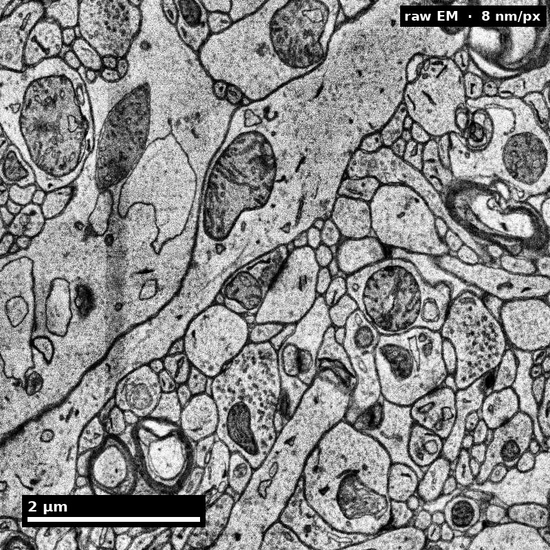
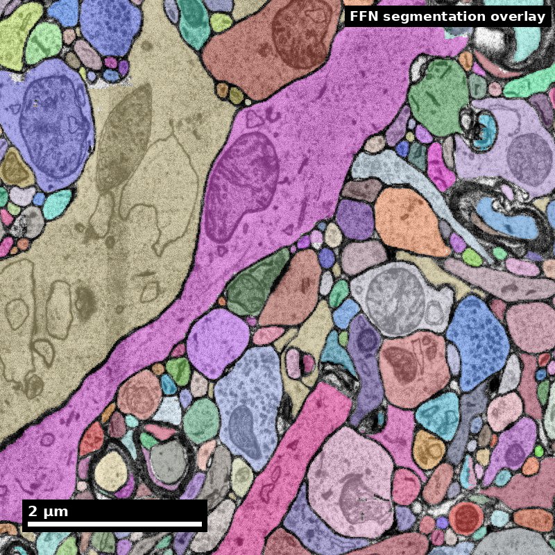
Now every voxel has to be assigned to the cell it belongs to. H01 used flood-filling networks (FFN) — a recurrent convolutional approach that grows one object at a time from a seed, repeatedly asking whether each neighbouring voxel belongs to the same object. Three FFN models were run, at 32, 16 and 8 nm, and their outputs combined into base segments which were then agglomerated.
Here is what that produces on one field — raw data, then the automated segmentation:
The two error modes are not symmetric
- A split breaks one true cell into several segments. Conservative: you under-report connectivity.
- A merge fuses two different cells. Far worse: it invents connections that do not exist and can contaminate a cell’s entire reported connectivity.
H01 ships two agglomerations, and the difference between them is this trade-off:
| c2 | c3 | |
|---|---|---|
| Character | fewer breaks, longer processes | conservative, shorter fragments |
| Merge corrections needed per cell | 400 | 257 (1.6× fewer) |
| Split corrections needed per cell | 238 | 504 (2.1× more) |
| Used for the paper’s analyses | no | yes |
Merge errors in the base segmentation were genuinely rare — 13 of 365,404 base segments, or 0.0036% — but agglomeration is where merges get introduced, which is why two versions exist at all. Automated cuts using a six-class subcompartment model (axon, dendrite, soma, astrocyte, axon initial segment, cilium) removed millions of suspect edges. Skeletonisation used kimimaro.
Step 7 — Synapse detection
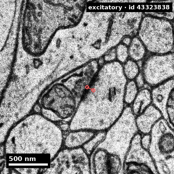
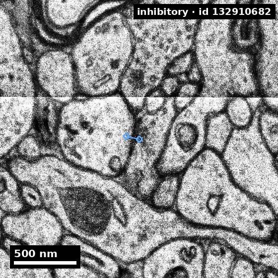
Segmentation says where cells are. It does not say where they talk. Synapse detection is a separate model — a 3D U-Net trained to find synaptic contacts, assign pre- and postsynaptic partners, and classify the presynaptic terminal as excitatory or inhibitory.
It found 149,871,669 synapses. Of the 133.7 million whose postsynaptic side was analysed, 99.4% land on dendrites, 0.39% on somata, and 0.20% on the axon initial segment.
Here are two real ones, drawn at their exact released coordinates:
Know the error rates before you use these numbers
| Excitatory | Inhibitory | |
|---|---|---|
| Missed (false negatives) | 11% | 35% |
| False discovery rate | 3.2% | 2.7% |
| E/I classification accuracy | 86.89% | 84.98% |
Inhibitory synapses are missed three times more often than excitatory ones. That single asymmetry should change how you read any E/I ratio computed from raw H01 counts. The authors correct for it: after adjusting for false discovery, false negatives and misclassification, they estimate 111.6 M excitatory (61.2%) and 70.7 M inhibitory (38.8%) — a substantially different balance from the raw classifier output.
Errors also compound across stages: a synapse detected correctly but attached to a merged segment gets reported as a connection onto the wrong cell.
Step 8 — Cell types, layers, and structure
With cells segmented and synapses attached, the volume can be organised anatomically.
57,180 cells: 49,080 neurons and glia, plus 8,100 blood-vessel-related cells.
| Count | |
|---|---|
| Glia | 32,315 |
| Neurons | 16,087 |
| — of which spiny (mostly pyramidal) | 10,531 (65.5%) |
| — of which non-spiny (interneurons) | 4,688 (29.1%) |
| Oligodendrocytes (most common cell type) | 20,139 |
| Astrocytes | 5,474 |
| Microglia | 2,517 |
| Endothelial cells | 4,604 |
Glia outnumber neurons 2:1, and neuron density is about 16,000/mm³ — roughly a third lower than light-microscopy estimates for human temporal cortex, and nearly tenfold lower than mouse association cortex.
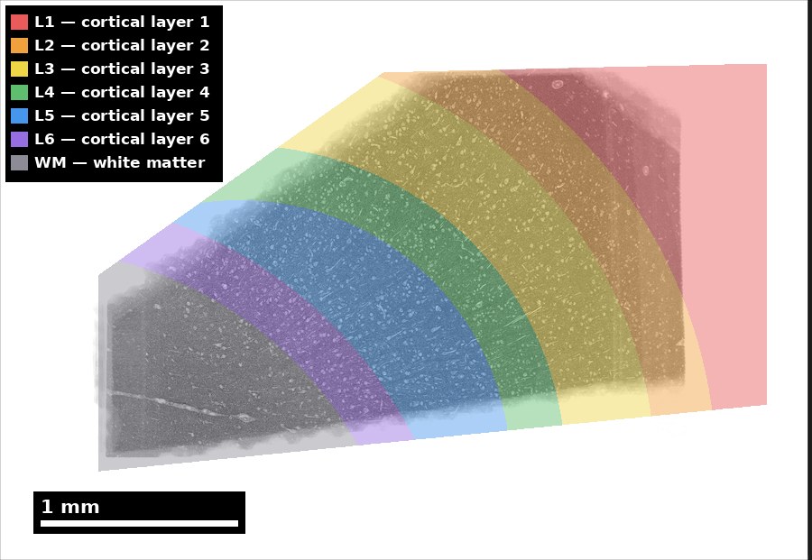
Layer boundaries were not drawn by hand: they were derived by clustering neurons on soma size and position, then fitting the resulting boundaries as arcs. That yields six layers plus white matter:
Step 9 — Proofreading
Automated reconstruction is not the end. Someone has to check it.
H01’s release includes 104 randomly-selected neurons proofread — every split and merge error in their axons, dendrites and somata corrected — distributed as meshes, skeletons, subcompartment labels and SWC reconstructions.
Two things about that number:
- 104 of 16,087 neurons. The paper is blunt that “it is infeasible for a single lab to proofread the entire dataset manually.”
- Dendritic spines were not proofread, even on those 104 cells — there are hundreds of thousands of them. On the one layer-2 pyramidal neuron where spines were checked, about a third were detached from their parent cell in the automated segmentation (32.2% in c2, 33.7% in c3 — the two agglomerations barely differ here).
Wider proofreading continues through CAVE, a collaborative web-based platform seeded from the c3 agglomeration, where anyone can apply to become a proofreader and the current proofread volume is browsable without applying. The release also ships CREST, a tool for exploring and correcting reconstructions.
The practical rule: if your question depends on one cell's complete and correct morphology, use a proofread cell or proofread it yourself. If your question is statistical across many cells, automated segmentation may be adequate — but you must reason about how split and merge rates bias your specific measurement, in your specific direction. And if your question involves spines, assume a third of them are detached until you check.
Step 10 — What they found
The neuropil is mostly not neurons, and mostly not cell bodies. By volume: unmyelinated axons ~40.2%, dendrites ~25.8%, glial processes ~15.5%, somata ~9.4%, myelinated axons ~7.5%. Glia outnumber neurons 2:1 and oligodendrocytes are the single most common cell type.
Deep-layer neurons come in mirror-image pairs. In layers 5 and 6, 876 “triangular” neurons — about a third of the spiny neurons there — have a large basal dendrite emerging at a wide angle from the apical dendrite. Their orientations are bimodal: 347 point “forward”, 339 point “reverse”, in mirror-symmetrical arrangement, along the anterior–posterior axis of the temporal lobe. Neighbouring triangular cells point the same way more often than chance (p = 0.005). The authors are careful to say what this means: “What the function of this bimodal distribution signifies remains unknown.”
Amid overwhelmingly weak connectivity, a few connections are extraordinarily strong. The distribution of synapses per axonal input is stark:
| Synapses from one axon onto one target | Share of connections |
|---|---|
| 1 | 96.49% |
| 2 | 2.99% |
| 3 | 0.35% |
| 4 or more | 0.092% |
And yet 39% of well-innervated neurons had at least one input making 7 or more synapses. In one proofread layer-3 pyramidal neuron with 397 postsynaptic partners, 97.5% of partners received between one and four synapses — but at eight sites where its axon crossed the dendrites of a single nearby inhibitory interneuron, it made 53 synapses onto that one partner. Against a null model where axons synapse freely on any dendrite within reach, this pattern is inconsistent with random partnering (p < 10⁻¹⁰, across 79.8 million axons).
Morphologically, these strong connections usually did not come from an axon running alongside a dendrite. More often the axon crossed without deviating, then sent terminal branches back to the same target on both sides of the crossing — sprouting up and down to the same partner.
The authors’ own framing: amid “a large number of exceedingly weak incidental connections,” cortical neurons are innervated by a small subset of inputs that “intentionally establish significantly more powerful connections.” And a caveat they attach themselves: because this used the uncorrected c3 data with many axonal splits, it likely underestimates connection strength. These are lower bounds.
Oddities with no established explanation. The dataset contains some extremely large spines, axon varicosities filled with unusual material, and a small number of axons forming extensive whorls. The authors note these have not been identified in neuropathological studies, and that “at present we are unable to determine whether they result from a pathological process, or are simply just rare.” More are catalogued in the H01 gallery.
Step 11 — What you should not conclude
The authors are explicit about the limits. The honest reading:
- This is not “the normal human cortex.” It is one cubic millimetre, from one person, with drug-resistant epilepsy. The authors: “we cannot exclude the possibility that long-term epilepsy, or its pharmacological treatment, had subtle effects on the nanometer-scale structure of the sample.” The reconstructed piece looked normal by light microscopy — that is a meaningful check, not a guarantee.
- Normality can only be established by comparison, and those comparisons do not exist yet: “Only by comparing samples obtained from patients with different underlying disorders may we eventually learn whether this sample is normal.” Note also that fresh samples from completely healthy people are “unlikely to ever be available” through neurosurgery.
- Inter-individual variability is unknown. As calibration, the authors point out that between individual C. elegans with identical genomes, 40% of neuron-to-neuron connectivity differs. Human association cortex is shaped by experience.
- Most of the volume is unvalidated. 104 cells are proofread. Some errors always remain, because removing split errors adds merge errors — that trade-off is not solved, it is chosen.
- Inhibitory connectivity is measurably less reliable than excitatory: 35% of inhibitory synapses were missed.
- A cubic millimetre truncates almost everything. Axons and dendrites leave the box. Connections you cannot see are not connections that do not exist.
- Structure constrains function; it does not reveal it. A wiring diagram says what can happen, not what does. The authors note that approaches to extracting meaning from connectivity data are “in their infancy.”
None of this makes H01 less valuable. It makes it a first human cubic millimetre rather than a definitive one.
Explore it yourself
- H01 release site — the official hub, with curated Neuroglancer views of pyramidal neurons, interneurons, astrocytes and oligodendrocytes on its Explore page.
- Gallery — a tour of the unusual structures found in the volume, whorls included.
- Released data — every layer
with its exact
gs://path, and the licence. - Code — the actual software used at each stage above.
How the figures on this page were made
Every EM figure here was rendered in this repository from the public volume, not copied
from a publication. The method is short enough to reproduce, and the same approach works
on any Neuroglancer precomputed dataset — MICrONS and FlyWire included.
Reading it needs a library that understands sharded precomputed data; TensorStore is used here, and CloudVolume is the common alternative:
import tensorstore as ts

vol = ts.open({
    'driver': 'neuroglancer_precomputed',
    'kvstore': {
        'driver': 'http',
        'base_url': 'https://storage.googleapis.com/h01-release/data/20210601/4nm_raw/',
    },
    'scale_metadata': {'key': '4.0x4.0x33.0'},   # native 4 x 4 x 33 nm
}).result()

# a 1024 x 1024 window from one section, at full resolution
tile = vol[614400:615424, 307200:308224, 2560, 0].read().result()
The zoom ladder is the same call against coarser scale_metadata keys. The segmentation
overlay reads .../c2/ at a matching scale and colours by segment ID. The synapse markers
come from the dataset’s own annotation layer (.../c2/synapses/precomputed), whose
spatial0 index holds a volume-wide sample of annotations carrying excitatory/inhibitory
labels and pre/post coordinates.
The full generator lives at scripts/render_h01_figures.py in this repository — run it
to regenerate every figure on this page from scratch.
Licence and attribution. All imagery on this page is derived from the H01 dataset, which the release site licenses as Creative Commons Attribution 4.0 ("All released datasets are licensed under a Creative Commons Attribution 4.0 License"). Dataset: the Lichtman Laboratory, Harvard University, and the Connectomics at Google team. Please cite: Shapson-Coe, A. et al. "A petavoxel fragment of human cerebral cortex reconstructed at nanoscale resolution." Science 384, eadk4858 (2024). doi:10.1126/science.adk4858. Note that the bioRxiv preprint carries a different, more restrictive licence than the dataset — do not conflate the two.