Slide 1 of 39
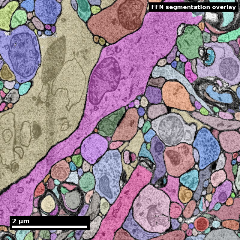
Synapse Detection
A graduate lecture from the NeuroTrailblazers reference layer
NeuroTrailblazers · neurotrailblazers.org
Part A — Three problems and the published record
Part B — Benchmarks and the sign problem
Part C — Using somebody else's synapse table
Human cortex · H01
Object segmentation over electron microscopy
H01 release · Lichtman Lab / Harvard & Connectomics at Google
Image: CC BY 4.0 · Shapson-Coe et al. (2024) · doi:10.1126/science.adk4858
Lecture: CC BY-SA 4.0 · neurotrailblazers.org
Figure description and teaching notes
This lecture is built from one page of the NeuroTrailblazers content library,
"Synapse Detection", and every number on these slides comes from that page and the
papers it cites. If you are adapting it, the page is the place to check a figure.
The goal is not that the room leaves able to train a detector. It is that they leave
able to download somebody else's synapse table and say what it can and cannot support.
Slide 2 of 39
The edges come from a detector
A connectome is a graph, and every edge in it was put there by a synapse detector
Everything downstream inherits whatever that detector got wrong:
- connection weights
- motif counts
- cell-type fingerprints
- connectome-constrained models
What this lecture is. The argument behind the one line a pipeline diagram gives this stage: what the task is, what has been tried, what the published numbers are, and what you have to measure before you are entitled to use somebody else's synapse table.
What it is not. Synapse biology — what a synapse is and how to recognise one by eye — is assumed, not taught.
Slide 3 of 39
Learning objectives
By the end of this lecture you will be able to:
1 — Distinguish localisation, partner assignment and sign classification as separate problems that succeed and fail independently.
2 — Interpret a published detector number by the unit it was measured at — synapse, interface, partner pair, or connection.
3 — State what a CREMI score does and does not predict about performance on your data.
4 — Explain how class-specific recall biases an excitatory/inhibitory ratio, and how much confidence a published correction deserves.
5 — Audit a released synapse table before building a claim on it.
Objective 4 is the one this lecture is really about. The single most consequential number in it is a recall figure, not an accuracy figure.
Slide 4 of 39
Roadmap
Part A — Three problems and the published record Why "synapse detection" is three tasks, what has been tried since 2011, and how to read a table of numbers that are not on a common scale.
Part B — Benchmarks and the sign problem What CREMI measures and what it cannot; WASPSYN and the domain-shift problem; why excitatory versus inhibitory is the hardest of the three tasks.
Part C — Using somebody else's synapse table A worked judgement on H01's excitatory/inhibitory balance; why detectors do not transfer; the checklist to run before trusting a table.
Bring to each part: a synapse table you have used or plan to use. By the end you should be able to say what its recall is in your region — or that nobody knows.
Slide 5 of 39
Synapse detection performance depends on the claim
Established methods can perform well in evaluated tissue. Localization, partner assignment and transfer still need separate validation.
Before the next slide: if a detector has 88% precision and recall per synapse, what do you expect its accuracy to be on the connectome built from it?
Figure description and teaching notes
Take answers, then explain that 88% per synapse is insufficient to predict an
edge-level score. Contact multiplicity, thresholds and correlated errors matter.
SynEM's results illustrate this distinction, not a universal conversion rule.
Slide 6 of 39
Established detection methods
Validation is specific to tissue, task and operating point
SynEM reports binary-connectome performance around 97% precision and recall. Its roughly 88% per-synapse result uses a different operating point.
Table 3 varies detector and connection thresholds. These numbers are not an automatic conversion.
H01's pipeline detected 149.9 million synapses at a 3.2% / 2.7% false-discovery rate (excitatory / inhibitory).
A published score does not certify a new table.
Measure detection and partner errors in the tissue and region supporting your claim.
Staffler et al. 2017 (10.7554/eLife.26414, SynEM); Shapson-Coe et al. 2024 (10.1126/science.adk4858, H01).
Figure description and teaching notes
Use Staffler et al. Table 3, not an implied 88-to-97 transformation. The same trained
model can be operated at different score thresholds and connection rules. Local
validation is still required. Ask whether the student's endpoint counts contacts
or asks only whether a neuron pair is connected.
Slide 7 of 39
The three residuals
What a table audit needs to establish
1 — Recall is not symmetric. H01's detector missed 11% of excitatory and 35% of inhibitory synapses. Unequal detection recall biases raw class counts; binary-edge performance does not repair a count ratio.
2 — Partner assignment is weaker than localisation, and much weaker where synapses are polyadic. Buhmann et al. report F1 from 0.59 to 0.73 across four areas of the same fly brain.
3 — Transfer is the operational cost. A detector trained on one volume does not move to another without new ground truth. As of 2025, the cross-dataset benchmarks say this is still open.
The honest budget line is not "we must solve synapse detection". It is: run the established detector, then spend your effort establishing what its recall and partner accuracy are in your region, and report the table's provenance.
Figure description and teaching notes
Residual 3 is why the NeuroTrailblazers open-problems list titles this problem
"Synapse detection that generalizes" rather than "synapse detection". The distinction
is the whole point of the lecture.
Slide 8 of 39
Part A
Three problems and the published record
- Localisation, partner assignment, sign
- What has been tried, with numbers
- Reading numbers that are not on a common scale
Slide 9 of 39
Three problems, not one
"Synapse detection" names at least three tasks that succeed and fail independently
1 — Localisation. Find the synapse. Depending on the method: segment the synaptic cleft as a set of voxels, predict a point annotation for the presynaptic site, or classify the interface between two already-segmented processes as synaptic or not.
2 — Partner assignment. Given a synapse, say which segment is presynaptic and which postsynaptic. A separate learning problem: Buhmann et al. (2021) and Turner et al. (2020) each treat it as its own network; Huang et al. (2018) use a U-Net for presynaptic sites and a separate multilayer perceptron, conditioned on the local segmentation, for postsynaptic partners.
3 — Sign or type. Excitatory or inhibitory. In mammalian cortex this is read from postsynaptic-density morphology; in Drosophila, from transmitter identity predicted from ultrastructure (Eckstein et al., 2024). The hardest of the three — Part B.
Slide 10 of 39
Two structural facts that change the shape of the problem
Insect synapses are polyadic. One presynaptic site contacts several postsynaptic partners, so "one cleft" is not "one edge".
Huang et al. (2018) describe theirs as "a complete solution for polyadic synapse detection"; the WASPSYN annotations record pre- and post-synaptic coordinates "together with their one-to-many connectivity information" (Li et al., 2024).
Some methods need a segmentation first; some do not. SynEM classifies borders between already-segmented processes; Heinrich et al. (2018) segment clefts directly from the raw image.
That decides whether segmentation errors propagate into your synapse table — and it means the two methods' F-scores are not measuring the same object.
Figure description and teaching notes
The second fact is the one people miss. An interface classifier works on borders
between segments the segmentation already produced, so whether segmentation errors
propagate into the synapse table depends on this choice -- and an F-score from one
kind of method is not directly comparable with an F-score from the other.
Slide 11 of 39
What has been tried, 2011–2018
| Method | Year | What it predicts | Reported performance | Tissue and preparation |
|---|---|---|---|---|
| ilastik (Kreshuk et al.) | 2011 | Asymmetric (presumed excitatory) synapse segmentation from voxel features | 0.92 recall at 0.89 precision on 111 validation synapses, "comparable to that of the experts" (three annotators) | Adult mammalian cortex, FIB/SEM, near-isotropic |
| Context cues (Becker et al.) | 2013 | Synapse segmentation plus synaptic orientation | Evaluated on three datasets; recovers orientation as a by-product | EM stacks, mixed |
| SyConn (Dorkenwald et al.) | 2017 | Synapses and types, alongside mitochondria, compartments, cell types | Framework paper; used to compute songbird basal-ganglia wiring | SBEM: zebrafish, mouse, zebra finch |
| SynEM (Staffler et al.) | 2017 | Neurite-interface classification: synaptic vs not | 88% / 88% per synapse; 94% / 89% spine synapses; 97% / 97% binary cortical connectomes | Mouse cortex, en-bloc staining, SBEM |
| 3D U-Net cleft (Heinrich et al.) | 2018 | Cleft voxels, by regression on a signed distance transform | A significant improvement over the prior state of the art on CREMI | Adult Drosophila, anisotropic ssTEM; ~50 teravoxels of whole fly brain |
| Huang et al. | 2018 | Presynaptic sites (U-Net) + postsynaptic partners (MLP) | Introduced connectome-scale evaluation metrics; most connectivity characterised correctly | Drosophila, polyadic |
Slide 12 of 39
What has been tried, 2020–2025
| Method | Year | What it predicts | Reported performance | Tissue and preparation |
|---|---|---|---|---|
| Attentional voxel association (Turner et al.) | 2020 | Pre- and postsynaptic masks, from a cleft mask used as an attention gate | Evaluated as part of a combined cleft-plus-partner system | Mouse somatosensory cortex |
| Synful (Buhmann et al.) | 2021 | Synaptic partners directly, whole brain | F1 0.73, 0.68, 0.66, 0.59 in four brain areas; 244 million putative partners from FAFB; 92–96% of edges correctly sorted weak (<5) vs strong (≥5) | Adult Drosophila, FAFB ssTEM |
| Cerebellar contact classifier (Park et al.) | 2022 | Synaptic vs not, plus pre/post side and E/I type | F1 = 0.955 on a test volume with 508 synapses | Mouse cerebellar molecular layer |
| H01 detector (Shapson-Coe et al.) | 2024 | Three-class U-Net + ResNet-50 E/I classifier | E and I recall differ by more than threefold — Part B | Human temporal cortex, ssEM 4 × 4 nm, 33 nm sections |
| SimpSyn (Mohinta et al.) | 2025 | Dual-channel spherical masks at pre- and postsynaptic sites, single-stage residual U-Net | Beats Synful in F1 on all volumes of a four-dataset invertebrate benchmark; generalisation across datasets remains limited | Adult and larval Drosophila, Megaphragma viggianii |
Full citations on the references slide. Every figure here is as reported in the method's own paper.
Slide 13 of 39
Reading the table: the numbers are not on a common scale
| Method | Number | Unit | Tissue |
|---|---|---|---|
| Kreshuk | 0.92 / 0.89 | per synapse | near-isotropic FIB/SEM |
| SynEM | 88 / 88 | per interface | anisotropic SBEM |
| Buhmann | 0.59–0.73 | per partner pair | ssTEM |
A method that looks worse here may simply have been measured on a harder unit in harder tissue.
Never rank two detectors by numbers taken from their own papers.
Park et al.'s F1 of 0.955 is the highest number on the previous two slides. What would you need to know before calling it the best detector?
Figure description and teaching notes
Expected answers: the unit (synaptic vs non-synaptic contacts), the test-set size (508
synapses -- a test set of a few hundred carries visible sampling error), and the tissue
(mouse cerebellar molecular layer, one preparation). The three readings on this slide
apply to it as much as to anything else in the table.
Slide 14 of 39
Reading the table: aggregation is doing enormous work
SynEM, from above. Per-synapse and binary-connectome scores use different evaluation units. Table 3 also varies score and connection thresholds.
Multiple contacts can help recover an edge when some contacts are missed. False positives, error correlation and the connection rule also affect performance.
Synful, from the other side. Per-connection F1 of 0.59–0.73 — but 92–96% of edges correctly assigned to the weak/strong classes most analyses actually use.
The number you need is the one measured at the level of your claim.
For most connectomics, that is the edge, not the synapse.
The field's accounting has moved. Huang et al. (2018) observed that as segmentation improved, synapse annotation came to consume "upwards of 50% of total effort". That is roughly when synapse detection stopped being the pipeline's afterthought — and why the later methods are about partners and generalisation rather than finding clefts.
Slide 15 of 39
Check yourself
What must accompany a binary-connectome performance number?
Report the evaluation unit, tissue and operating point. Detector score thresholds and the number of contacts required to call an edge affect the result.
SynEM's Table 3 distinguishes thresholds optimized for contacts from those optimized for connections.
Quote the paper's result as that paper's result. Claiming the same performance on your table requires validation of its connection rule and domain.
Do not quote it for synapse counts, connection weights, or anything per-synapse.
Aggregation can change both precision and recall. It does not remove class-specific bias in synapse counts.
Slide 16 of 39
Part B
Benchmarks and the sign problem
- What a CREMI score does and does not tell you
- WASPSYN and the 0.001% ratio
- Excitatory versus inhibitory, and why it is harder
Slide 17 of 39
CREMI: the reference benchmark
Circuit Reconstruction from Electron Microscopy Images
The data. Three datasets, each two (5 µm)³ volumes — training and testing, 1250 × 1250 × 125 px — of serial-section TEM of the adult Drosophila brain at [4, 4, 40] nm. Each training volume ships neuron ids, synaptic-cleft segmentation, and (pre, post) partner pairs.
| CREMI task | How it is scored |
|---|---|
| Neuron segmentation | Variation of Information, Adapted Rand error, Tolerant Edit Distance |
| Synapse detection | F-measure over false positives and false negatives; a predicted cleft voxel beyond a threshold distance from any ground-truth cleft is a false positive, and vice versa |
| Connectivity (partner identification) | F-measure over matched (pre, post) pairs, matched by an assignment problem minimising Euclidean distance within a threshold |
What the scoring does not do: require a predicted cleft to overlap the ground truth voxel-for-voxel — only to fall within a distance tolerance. Cleft detection is localisation with slack, which is why methods that regress a distance transform (Heinrich et al., 2018) do well on it.
Figure description and teaching notes
The exact weighting that combines the components into a single CREMI ranking score is
deliberately not stated here: the source page could not recover it from the primary
source, and says so. If someone asks, that is the honest answer.
Slide 18 of 39
What a good CREMI score predicts — and what it does not
It predicts that your method is competitive on anisotropic fly ssTEM, at CREMI's resolution, under CREMI's convention for what counts as a cleft.
That is worth knowing. It is why CREMI training data underlies whole-brain fly cleft prediction: Heinrich et al. trained on CREMI's annotated crops, then predicted clefts across ~50 teravoxels of the complete Drosophila brain.
It does not predict:
- Performance elsewhere in the same volume. One Synful model: F1 0.73, 0.68, 0.66, 0.59 across four areas of one fly brain. A 0.14-point spread within one sample exceeds the gap between many published methods.
- Performance in mammalian tissue. Different voxel size, anisotropy, staining chemistry, synapse geometry — and no polyadic structure to exploit.
- Whether your edges are right. Connectivity is scored on pairs, not the weighted graph you will use.
- Inhibitory recall. CREMI does not separate sign at all.
Slide 19 of 39
WASPSYN: the benchmark built to measure what CREMI cannot
Domain adaptation, as a benchmark. Li et al. (2024) annotated 14 image volumes from a biologically diverse set of Megaphragma viggianii brain regions, drawn from three different whole-brain datasets, and ran it as an ISBI 2023 challenge.
The number that defines the problem.
Manual annotation is so expensive that labelled training data is "often smaller than 0.001% of the large-scale image volumes in application".
That ratio, not any single F1, is why cross-dataset generalisation is the live question. 0.001% is one part in 100,000: a detector is applied to volumes five orders of magnitude larger than anything it was shown labelled.
Figure description and teaching notes
No CREMI or WASPSYN leaderboard position is quoted anywhere in this lecture.
Leaderboards move; the numbers here come from papers that can be re-checked.
Slide 20 of 39
Check yourself
A team beats the published CREMI cleft F1. What have they demonstrated, and what have they not?
Demonstrated
Competitiveness on anisotropic adult-fly ssTEM at 4 × 4 × 40 nm, under CREMI's annotation convention and distance-tolerant scoring.
Not demonstrated
- mammalian tissue
- other regions of a fly brain (0.59–0.73 within one brain)
- sign classification
- the accuracy of the weighted graph a user would build
Which of the four "not demonstrated" items would matter most for a study of cortical E/I balance? Hold it — the next four slides answer it.
Slide 21 of 39
Excitatory versus inhibitory: why it is harder
Cleft detection asks "is there a synapse here?" Sign asks "what kind?" — on thinner evidence
The morphological basis is a statistical mapping, not a rule. Synapses sort into Gray's type I and type II, corresponding to Colonnier's asymmetric (AS) and symmetric (SS): AS have a thick postsynaptic density, SS a thin one.
In cerebral cortex most AS are excitatory (glutamatergic) and most SS inhibitory (GABAergic) — "most", not all.
Validation is possible, and has been done. Cano-Astorga et al. (2024) check the morphological call against molecular markers, using immunocytochemistry for the vesicular GABA transporter to confirm that symmetric synapses seen under their protocol are GABAergic.
Slide 22 of 39
The discriminating feature is a few voxels thick — and staining moves it
Potassium ferrocyanide is used in modern volume-EM protocols to enhance membrane contrast.
Cano-Astorga et al. (2024) show that as its concentration rises, postsynaptic densities get thinner, so symmetric synapses become progressively harder to identify. They recommend 0.1%.
The consequence for a detector is stark.
The feature your inhibitory classifier depends on is partly a property of the sample-preparation recipe, not only of the tissue.
A classifier trained on one lab's staining is being asked to transfer across chemistry, not just across brains.
Figure description and teaching notes
This is the mechanism behind residual 1. It is not that inhibitory synapses are
inherently invisible; it is that the one feature separating them from excitatory ones
is thin, and a routine contrast-enhancing reagent thins it further.
Slide 23 of 39
The asymmetry, in H01's own numbers
From manual proofreading of a selection of axons across all cortical layers (Shapson-Coe et al., 2024)
| Excitatory | Inhibitory | |
|---|---|---|
| False negatives (missed synapses) | 11% | 35% |
| False discovery rate | 3.2% | 2.7% |
| Correctly classified as this type | 86.89% | 84.98% |
Precision is excellent and near-identical for both classes. Recall is not. The detector misses roughly one inhibitory synapse in three, and one excitatory synapse in nine.
That single asymmetry is the most consequential number in this lecture. Part C works out what it does to a result.
Figure description and teaching notes
Point at the FDR row first, then the false-negative row. The FDR row is what a
precision-focused evaluation shows you, and it looks reassuring. The false-negative
row is the one that bites, and it is the one a single combined F1 would hide.
Slide 24 of 39
In insects, sign is a different problem entirely
Fly synapses do not give up their sign through AS/SS morphology, so the question becomes transmitter identity.
Eckstein et al. (2024) trained networks on EM images at synaptic sites to predict six transmitters — acetylcholine, glutamate, GABA, serotonin, dopamine, octopamine — across a whole Drosophila brain.
| Level | Accuracy |
|---|---|
| Individual synapses | 87% |
| Neurons | 94% |
| Known cell types | 91% |
The 87 → 94 step is the aggregation effect again: a neuron's synapses vote.
Which has a consequence. Fly connectome signs are, in practice, properties of neurons. Treating per-synapse predictions as independent evidence double-counts.
Slide 25 of 39
Part C
Using somebody else's synapse table
- A worked judgement: H01's excitatory/inhibitory balance
- Why detectors do not transfer
- The checklist, and bounding your own risk
Slide 26 of 39
Take the H01 synapse table as released.
What fraction of synapses in human temporal cortex are excitatory?
You have the table and a laptop. Write down the number you would put in a paper, and the sentence you would put next to it.
Figure description and teaching notes
Give them a minute. Almost everyone will propose computing the ratio from the table.
That is the right first step and the wrong final answer, and the next four slides are
why.
Slide 27 of 39
The straight count, and the corrected estimate
The straight count. Shapson-Coe et al. report 149,871,669 synapses automatically detected:
| Count | Share | |
|---|---|---|
| Excitatory | 111,272,315 | 74.2% |
| Inhibitory | 38,599,354 | 25.8% |
If you pull the released table and compute a ratio, this is your answer.
The corrected estimate. The authors do not report that number as their result. Adjusting for the measured false-discovery, false-negative and misclassification rates, they estimate:
| Estimate | Share | |
|---|---|---|
| Excitatory | 102.5 M | 67.1% |
| Inhibitory | 50.3 M | 32.9% |
Slide 28 of 39
What moved
Almost all of it is the 35% inhibitory false-negative rate
Precision was fine for both classes, so few detected synapses are spurious. The problem is the ones never detected — and they are disproportionately inhibitory.
Running the arithmetic the other way:
- Raw table: 38.6 M of an estimated 50.3 M inhibitory — short by about 23% of the inhibitory population.
- Raw excitatory count of 111.3 M sits about 9% above the 102.5 M estimate.
The naive ratio is wrong in both directions at once.
That is why the error on the ratio — 74.2% versus 67.1%, or 7.1 percentage points — is larger than the error on either count alone.
Figure description and teaching notes
Walk the arithmetic on the board if there is time: 38.6 / 50.3 is about 0.77, so 23%
short; 111.3 / 102.5 is about 1.09, so 9% over. The source attributes almost all of
the shift to the 35% inhibitory false-negative rate; do not improvise a finer
breakdown of the excitatory overcount than the paper's correction gives.
Slide 29 of 39
How confident should you be in the correction?
Less than in the raw count
The correction rests on proofreading a selection of axons, not a dense re-annotation. So:
- the rates carry their own sampling error
- they were measured across cortical layers that differ in inhibitory density
The corrected figure is an estimate from a sample.
The raw figure is an exact count of a biased measurement.
Neither is "the number of synapses in the tissue" — and a paper quoting either without saying which has not told you what it did.
Figure description and teaching notes
This is the slide where the caveat must not be dropped for punchiness. The corrected
67:33 is better-motivated than 74:26, but it is not ground truth either. The correct
sentence names which number it is and where it came from.
Slide 30 of 39
What follows, well beyond H01
1 — Any excitation/inhibition ratio computed straight from a released synapse table is biased toward excitation, by an amount set by the detector's class-specific recall. Report the recall figures alongside the ratio, or do not report the ratio.
2 — Comparisons are safer than absolutes. For two regions processed by the same detector and staining, the difference in E/I ratio survives a shared bias that the absolute value does not.
3 — The bias is not random, so more data will not fix it. Ten times the volume buys ten times the confidence in the wrong number.
Back to the cold open. A defensible sentence: "74.2% of automatically detected synapses were classified excitatory; the authors' correction for class-specific detection rates, estimated from proofread axons, gives 67.1%." Two numbers, both labelled.
Slide 31 of 39
Why detectors do not transfer
Every one of these differs between two EM volumes, and every one can move a detector's output
| What changes | Concrete example |
|---|---|
| Voxel size and anisotropy | CREMI/FAFB at 4 × 4 × 40 nm ssTEM; H01 at 4 × 4 nm in-plane with 33 nm sections; FIB/SEM near-isotropic. Heinrich et al. built a 3D U-Net specifically "to optimally represent isotropic fields of view in non-isotropic data" — the architecture itself encodes an assumption about the sampling grid |
| Staining chemistry | Potassium ferrocyanide concentration changes apparent PSD thickness (Cano-Astorga et al., 2024) — directly attacking the inhibitory-synapse feature |
| Species ultrastructure | Polyadic insect synapses versus predominantly monadic mammalian ones; the output structure differs, not just the appearance |
| Annotation convention | What counts as a cleft, and where a "site" point sits relative to it. Two ground-truth sets can disagree systematically while both being correct by their own rules |
| Region within one sample | Buhmann et al.: F1 0.59 to 0.73 across four areas of the same fly brain |
Slide 32 of 39
The honest summary is narrower than "models do not transfer"
Within a volume and preparation, spatial generalisation is often fine. Heinrich et al. report that their model, trained on CREMI's small annotated crops, "generalizes well to areas far away from where training data was available" — across a whole fly brain, including lamina.
Across preparations, it is not.
- SimpSyn: across four invertebrate datasets, generalisation remains limited even for the model that wins within each.
- SynapseNet built explicit domain-adaptation functionality in rather than relying on a large training set.
- WASPSYN exists because methods that "utilize in-domain labeled data and generalize to out-of-domain unlabeled data are in urgent need".
The distinction is operational.
Analysing one released volume? Its detector was probably trained on that volume; the within-sample evidence applies to you.
Bringing a published detector to new tissue? You are in the regime where the evidence says it will degrade — by an amount nobody can tell you in advance.
Slide 33 of 39
Before you trust a synapse table
You will usually not be running a detector. You will be downloading a table someone else's produced.
| Ask | Why it changes what you can claim |
|---|---|
| Which detector, which version, which materialization? | Synapse tables are regenerated. A result that does not name the version is not reproducible |
| Ground truth: how many synapses, annotated by whom, with what agreement? | Kreshuk et al.: 111 synapses, three experts. SynEM's test set: 235 synapses among 20,319 non-synaptic interfaces. A test set of a few hundred carries visible sampling error |
| Per synapse or per connection? | SynEM: 88% versus 97%. Both true; different questions |
| Precision and recall reported separately for E and I? | H01: 3.2% versus 2.7% FDR, but 11% versus 35% false negatives. A single combined F1 hides exactly the error that will bite you |
| Stratified by region? | Buhmann et al.: 0.59 to 0.73 within one brain. A whole-volume average tells you nothing about your region |
| Polyadicity convention: one row per site, or per (pre, post) pair? | Miscounting this inflates or deflates every insect connection weight |
| What distance tolerance in the evaluation? | CREMI-style scoring matches within a threshold. A generous threshold flatters everything |
| Evaluated on the same preparation as your volume? | If not, the transfer problem applies and the published number is an upper bound at best |
Slide 34 of 39
If none of that is available: bound your own risk in an afternoon
The procedure. Take a random subvolume, annotate every synapse in it by hand, and compare against the table.
- missed table entries → recall
- spurious table entries → precision
Tooling. SynAnno (Lauenburg et al., 2025) provides guided, neuron-centric synapse proofreading with model-assisted error detection.
Two calibration points set expectations.
Kreshuk et al. found their algorithm's error rate "comparable to that of the experts". SynEM reports its expert annotators at 93.6–94.6% precision and 97.9–98.9% recall.
Agreement in the mid-90s is roughly what two competent humans achieve. A detector matching your annotations more closely than that should make you suspicious of your annotations, not confident in the detector.
Slide 35 of 39
Check yourself
You compute an excitatory:inhibitory ratio of 74:26 from H01's released table. Name the measurement that makes this wrong, and the direction.
The measurement. The 35% false-negative rate for inhibitory synapses, against 11% for excitatory.
The direction. The released table is short by roughly 23% of the estimated inhibitory population, so the ratio is biased toward excitation.
The authors' corrected estimate is 67:33 — about 7 percentage points away.
And the follow-up question worth asking of any answer: which number is it — the count of a biased measurement, or the estimate from a proofread sample? Both are legitimate. Unlabelled, neither is.
Slide 36 of 39
What this lecture does not cover
Boundaries stated deliberately, as the source page states them
- Synapse biology — what a synapse is, vesicle pools, active-zone architecture, spine types, recognition by eye.
- Neurite segmentation — affinities, watershed, agglomeration, flood-filling networks, and their error modes.
- The mathematics of the metrics — VI, ERL and the F1 family, derived.
- Gap junctions. A genuinely separate detection problem; no performance figures are quoted because none were sourced.
- Synapse size as a strength proxy. Cleft and PSD area are used throughout the literature to weight edges; assessing that calibration is a live open problem, not evaluated here.
- Leaderboard standings and the exact CREMI score formula. Leaderboards move; the precise weighting was not recovered from the primary source, so none is stated.
- Compute cost on current hardware. The only sourced throughput figures predate current accelerators by years. Do not plan a budget from them.
- Non-EM synapse mapping — array tomography, expansion microscopy, light-microscopy connectomics.
Slide 37 of 39
Where to go next
The source page. Synapse Detection in the NeuroTrailblazers content library — this lecture's full argument, with every number linked to its paper.
Neighbouring pages. Reconstruction pipeline (where this stage sits); Metrics and QA (the metric definitions); Synapse classification (the biology this lecture presupposes); Provenance and versioning (pinning the table you used); the H01 case study (the volume behind Part C).
Hands-on. Technical training Unit 08, segmentation and proofreading.
The one idea to carry forward.
Cleft detection is solved. What a synapse table can support is not a property of the detector — it is a property of its recall by class, its partner accuracy in your region, and whether it was evaluated on your preparation.
Measure those, or report that nobody has.
Slide 38 of 39
References and sources
Detection methods. Kreshuk et al. 2011 (10.1371/journal.pone.0024899, ilastik synapse detection); Becker et al. 2013 (10.1109/TMI.2013.2267747, context cues); Dorkenwald et al. 2017 (10.1038/nmeth.4206, SyConn); Staffler et al. 2017 (10.7554/eLife.26414, SynEM); Heinrich et al. 2018 (10.1007/978-3-030-00934-2_36, cleft segmentation in the complete Drosophila brain); Huang, Scheffer & Plaza 2018 (10.3389/fncir.2018.00087, fully-automatic synapse prediction); Turner et al. 2020 (10.1109/ISBI45749.2020.9098489, attentional voxel association); Buhmann et al. 2021 (10.1038/s41592-021-01183-7, Synful); Park et al. 2022 (10.3389/fnana.2022.760279, cerebellar synapse detection); Mohinta et al. 2025 (arXiv:2509.17041, SimpSyn).
Sign and transmitter identity. Cano-Astorga et al. 2024 (10.3389/fnana.2024.1348032, asymmetric and symmetric synapses in volume EM); Eckstein et al. 2024 (10.1016/j.cell.2024.03.016, neurotransmitter classification in Drosophila).
Datasets, benchmarks and tools. Shapson-Coe et al. 2024 (10.1126/science.adk4858, H01); CREMI challenge (cremi.org); Li et al. 2024 (10.1109/TMI.2024.3400276, WASPSYN); Muth et al. 2024 (10.1091/mbc.e24-11-0519, SynapseNet); Lauenburg et al. 2025 (10.1101/2025.08.09.669342, SynAnno).
Source page. NeuroTrailblazers content library, Synapse Detection (/content-library/infrastructure/synapse-detection/). https://neurotrailblazers.org
Slide 39 of 39
Use, adapt, and credit
These slides are openly licensed for community use
Licence: CC BY-SA 4.0
Creative Commons Attribution-ShareAlike 4.0 International.
https://creativecommons.org/licenses/by-sa/4.0/
You may teach from these slides anywhere, including commercially; copy and redistribute them in any medium; and re-cut, shorten, translate, restyle, or merge them into your own material — and distribute the result. No permission needed.
Two conditions. Attribution — credit the original, link the licence, and say if you changed anything. ShareAlike — distribute your adapted version under this same licence, so it stays as open as what it came from.
How to credit
NeuroTrailblazers (2026). Synapse Detection (graduate lecture, NeuroTrailblazers reference layer). CC BY-SA 4.0. neurotrailblazers.org/technical-training/slides/
For an adaptation, prefix with "Adapted from" and note what you changed.
Editable source. The Marp markdown is in the repository — the exported PowerPoint renders each slide as an image, so the markdown is the thing to edit. https://github.com/wrgr/neurotrailblazers
Improved something? The project would like to hear about it — open an issue.
Cover image: H01 release, Lichtman Lab / Harvard & Connectomics at Google, CC BY 4.0. Shapson-Coe et al. (2024), doi:10.1126/science.adk4858. The image retains its own licence. Cited papers carry their own licences; citation is not reproduction.